Arbitrary bosonic state preparation using smooth pulses : Gradient based dCRAB optimisation using GOAT over GRAPE method
In this example we solve the task in the previous example of preparing arbitrary bosonic state, but using smooth functions as the basis. Here we perform a gradient based dCRAB optimisation, by using the GOAToverGRAPE (or the GROUP [Sørensen2018]) method.
import numpy as np
import matplotlib.pyplot as plt

from paraqeet.quantity import Quantity
from paraqeet.model.resonator import Resonator
from paraqeet.model.qubit import Qubit
from paraqeet.model.coupling import Coupling
from paraqeet.signal.envelopes import DCRABEnvelope
from paraqeet.signal.pwc_generator import PWCGenerator
from paraqeet.model.closed_system import ClosedSystem
from paraqeet.model.rotating_frame_drive import RotatingFrameDrive
from paraqeet.model.composite_hamiltonian import CompositeHamiltonian
from paraqeet.measurement.state_transfer_fidelity import StateTransferFidelityGRAPE
from paraqeet.measurement.weighted_sum_goal import WeightedSumGoal
from paraqeet.propagation.scipy_expm_grape import ScipyExpmGRAPE
from paraqeet.optimisation_map import OptimisationMap
from paraqeet.measurement.goat_over_grape import GOATOverGRAPE
from paraqeet.optimisers.dcrab_optimiser_gradient import DCRABOptimiserGradient
from paraqeet.signal.waveform import FlatTopGaussianFilter
from paraqeet.file_logger import FileLogger
Following the dCRAB optimization [Müller2022], we initialize our pulses
in the frequency domain by using the DCRABEnvelope. Further we use a
flat-top Gaussian filter on top to ensure that the pulses start and end
at zero. And we use a PWCGenerator to generate the piece-wise
constant signal required for the GOAToverGRAPE method.
# in seconds (See Eickbusch et al https://arxiv.org/abs/2111.06414 S9 A)
delta_sampling = 33e-9
n_pwc = 40  # number of piecewise constants in the pulse
t_final = n_pwc * delta_sampling  # for now just set up for trying
tlist = np.linspace(0, t_final, n_pwc + 1)
eps_res = 3 * np.pi * 1.0  # initial amplitude of the resonator (in MHz)
eps_max_res = 5 * eps_res  # maximum amplitude of the resonator (in MHz)
eps_qubit = 3 * np.pi * 1.0  # initial amplitude of the qubit (in MHz)
eps_max_qubit = 5 * eps_qubit  # maximum amplitude of the resonator (in MHz)

tone_res = DCRABEnvelope(
    num_components=2,
    max_frequency=2 * np.pi * 2.0,
    amplitude=Quantity(eps_res * 1e6, -eps_max_res * 1e6, eps_max_res * 1e6, name="Amplitude CRAB resonator"),
    t_final=Quantity(t_final, 1 / 2 * t_final, 2 * t_final, name="t_final CRAB resonator"),
    seed=46874,
)

smooth_tone_res = FlatTopGaussianFilter(
    envelopes=tone_res, t_final=Quantity(t_final, 1 / 2 * t_final, 2 * t_final, name="t_final")
)

tone_qubit = DCRABEnvelope(
    num_components=2,
    max_frequency=2 * np.pi * 2.0,
    amplitude=Quantity(eps_qubit * 1e6, -eps_max_qubit * 1e6, eps_max_qubit * 1e6, name="Amplitude CRAB qubit"),
    t_final=Quantity(t_final, 1 / 2 * t_final, 2 * t_final, name="t_final CRAB qubit"),
    seed=189841,
)

smooth_tone_qubit = FlatTopGaussianFilter(
    envelopes=tone_qubit, t_final=Quantity(t_final, 1 / 2 * t_final, 2 * t_final, name="t_final")
)

gen_res = PWCGenerator(envelopes=[smooth_tone_res], tlist=tlist, max_amplitude=2 * eps_max_res * 1e6)
gen_qubit = PWCGenerator(envelopes=[smooth_tone_qubit], tlist=tlist, max_amplitude=2 * eps_max_qubit * 1e6)
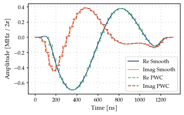
Here we plot the resonator tone and compare it to its smooth version. Similarly one can plot the qubit tone.
from plotting import plot_signal

ts = np.linspace(0, t_final, 1001)
fig, ax = plt.subplots(1, figsize=(5, 3))

plot_signal(smooth_tone_res, ts, ax, linestyle="-", label="Smooth")
plot_signal(gen_res, ts, ax, linestyle="--", label="PWC")

plt.legend()
plt.show()
Like the previous example, we define qubit and resonator parameters, as well as the list of different Fock truncation numbers. We also set the target Fock state.
For now we set the Fock-state truncation at small values (3 and 4) for testing the method. Later we demonstrate the method with (30 and 31) levels in the resonator.
# Increasing the number of Fock states gives a more realistic scenario, at the price of increasing the simulation time
n_fock_truncation_list = [3, 4]
fock_target = 2
n_times = 1001

omega_range_factor = 1e-3  # just for initialization of the Quantity object
omega_res = 2 * np.pi * 5.26e9
omega_qubit = 2 * np.pi * 6.65e9

omega_drive_res = omega_res
omega_drive_qubit = omega_qubit

detuning_drive_res = omega_res - omega_drive_res
detuning_drive_qubit = omega_qubit - omega_drive_qubit

drive_res = RotatingFrameDrive(gen_res)
drive_qubit = RotatingFrameDrive(gen_qubit)
Similar to the previous example, following [Heeres2017], we thus consider \(N_{\mathrm{T}} \in \{N_{\mathrm{T}}^{(\mathrm{min})}, N_{\mathrm{T}}^{(\mathrm{min})} + 1, \dots, N_{\mathrm{T}}^{(\mathrm{max})} \}\), and introduce a penalty when having different values of fidelities for different truncation numbers. Thus, we create different systems, and accordingly fidelity measures, for the different Fock truncation numbers.
def create_experiment(n_fock_truncation_list, fock_target):
    """
    Create the inital and target states, for the given Fock numbers.
    Also create the propagations and measurements for the given truncation numbers and target Fock states.
    """
    resonator_list = []
    coupling_list = []
    model_list = []
    hamiltonian_list = []
    prop_list = []
    initial_state_list = []
    target_state_list = []
    fock_number_op_list = []
    dcrab_fid_list = []

    qubit = Qubit(
        frequency=Quantity(
            value=detuning_drive_qubit,
            min_value=-omega_range_factor * omega_qubit,
            max_value=omega_range_factor * omega_qubit,
        ),
        drives=[drive_qubit],
    )
    ground_state_qubit = np.array([[0.0], [1.0]])

    # We take it to be 10 times the value in Eickbusch et al to speed up the simulation
    chi = 2 * np.pi * 32.81e3 * 10

    for n in n_fock_truncation_list:
        resonator = Resonator(
            frequency=Quantity(
                value=detuning_drive_res,
                min_value=-omega_range_factor * omega_res,
                max_value=omega_range_factor * omega_res,
            ),
            dimension=n,
            drives=[drive_res],
        )
        resonator_list.append(resonator)
        coupling = Coupling(
            [resonator, qubit],
            is_longitudinal=True,
            coefficient=Quantity(value=chi, min_value=chi / 2, max_value=2 * chi),
        )
        coupling_list.append(coupling)
        ham = CompositeHamiltonian([resonator, qubit], [coupling])
        hamiltonian_list.append(ham)
        model = ClosedSystem(hamiltonian=ham)
        model_list.append(model)
        prop = ScipyExpmGRAPE(model, res=1e9)

        initial_res_state = np.zeros([n, 1], dtype=complex)
        initial_res_state[0, 0] = 1  # vacuum state
        initial_state = np.kron(initial_res_state, ground_state_qubit)
        initial_state_list.append(initial_state)

        target_res_state = np.zeros([n, 1], dtype=complex)
        target_res_state[fock_target, 0] = 1
        target_state = np.kron(target_res_state, ground_state_qubit)
        target_state_list.append(target_state)

        n_op = np.kron(np.diag([x for x in range(n)]), np.identity(2))
        fock_number_op_list.append(n_op)

        prop.set_initial_state(initial_state)
        prop.target_state = target_state
        prop.use_schirmer_derivative = True

        prop_list.append(prop)

        fid = StateTransferFidelityGRAPE(
            propagation=prop, initial_state=initial_state, target_state=target_state, times=tlist
        )
        goat_over_grape_fid = GOATOverGRAPE(fid, generators=[gen_res, gen_qubit], generators_order=[0, 1])
        dcrab_fid_list.append(goat_over_grape_fid)

    return initial_state_list, target_state_list, fock_number_op_list, prop_list, dcrab_fid_list


initial_state_list, target_state_list, fock_number_op_list, prop_list, dcrab_meas_list = create_experiment(
    n_fock_truncation_list, fock_target
)
We consider as cost function of the form
that we want to maximize. This cost weighted cost function can be constructed using the class WeightedSumGoal.
Note - As we consider smooth pulses as our basis function, we do not need to add additional smoothness cost to the goal function.
weights = np.array([1.0 for _ in range(len(dcrab_meas_list))])
weight_sum_of_squares = -0.05
total_sum_of_weights = np.sum(weights) + weight_sum_of_squares
weights = weights / total_sum_of_weights
weight_sum_of_squares = weight_sum_of_squares / total_sum_of_weights
dcrab_meas_list_bool = [True for meas in dcrab_meas_list]
sum_of_squares_options = {"weight": weight_sum_of_squares, "meas_bool": dcrab_meas_list_bool}

dcrab_goal = WeightedSumGoal(dcrab_meas_list, weights, sum_of_squares_options=sum_of_squares_options)
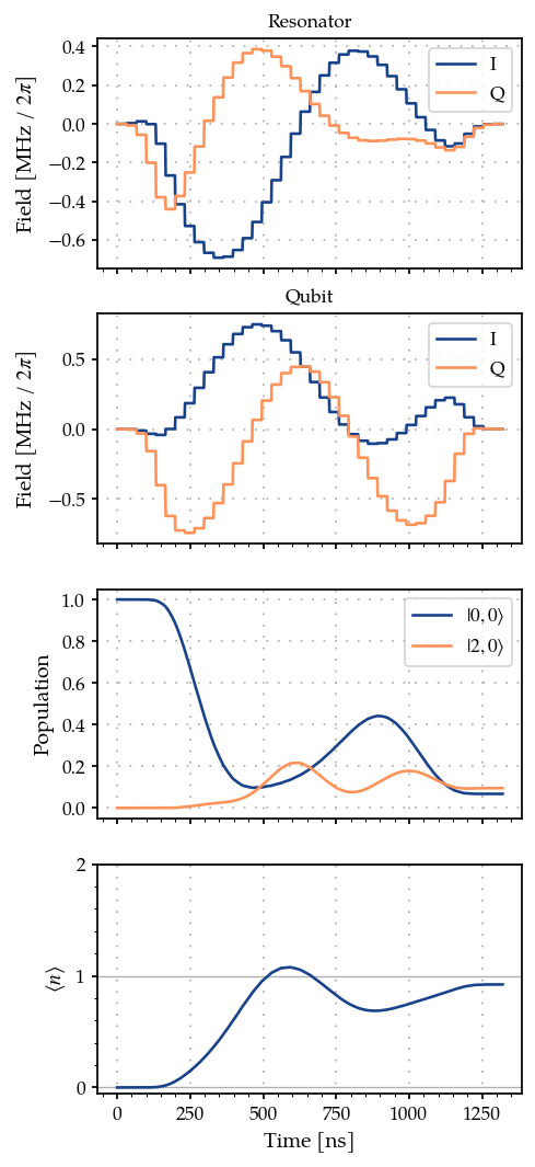
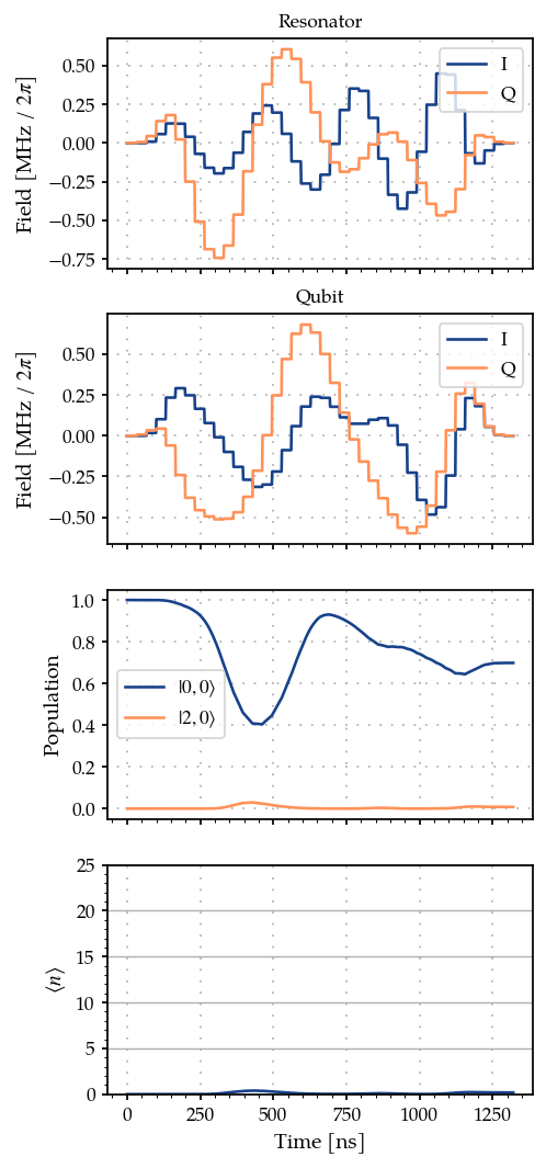
We can plot the initial pulses, as well as the corresponding relevant dynamics.
def plot_states_and_fock_number(item=0):
    """Plot the states."""
    ts = np.linspace(0, t_final, n_times)
    states = prop_list[item].propagate(ts)
    sig_res = gen_res.generate_signal(ts)
    sig_qubit = gen_qubit.generate_signal(ts)
    pop_initial_state = (np.abs(initial_state_list[item].conj().T @ states) ** 2).flatten()
    pop_target_state = (np.abs(target_state_list[item].conj().T @ states) ** 2).flatten()

    pop_initial_state = (np.abs(initial_state_list[item].conj().T @ states) ** 2).flatten()

    n_fock_avg = np.zeros(n_times, dtype=float)
    for k in range(n_times):
        n_fock_avg[k] = np.real((states[k].conj().T @ fock_number_op_list[item] @ states[k])[0, 0])

    _, ax = plt.subplots(4, figsize=(4, 10), sharex=True)
    ax[0].plot(ts / 1e-9, np.real(sig_res) / 1e6 / (2 * np.pi), label="I")
    ax[0].plot(ts / 1e-9, np.imag(sig_res) / 1e6 / (2 * np.pi), label="Q")
    ax[0].legend(loc=1)
    ax[0].set_ylabel(r"Field [MHz / $2\pi$]")
    ax[0].set_title("Resonator")
    ax[0].grid(True, linestyle=(1, (1, 5)), linewidth=1)

    ax[1].plot(ts / 1e-9, np.real(sig_qubit) / 1e6 / (2 * np.pi), label="I")
    ax[1].plot(ts / 1e-9, np.imag(sig_qubit) / 1e6 / (2 * np.pi), label="Q")
    ax[1].legend(loc=1)
    ax[1].set_ylabel(r"Field [MHz / $2\pi$]")
    ax[1].set_title("Qubit")
    ax[1].grid(True, linestyle=(1, (1, 5)), linewidth=1)

    ax[2].plot(ts / 1e-9, pop_initial_state, label="$|0,0 \\rangle$")
    ax[2].plot(ts / 1e-9, pop_target_state, label="$|2, 0 \\rangle$")
    ax[2].legend(loc="best")
    ax[2].set_ylabel("Population")
    ax[2].grid(True, linestyle=(1, (1, 5)), linewidth=1)

    ax[3].plot(ts / 1e-9, n_fock_avg)
    ax[3].set_ylabel("$\\langle n \\rangle$")
    if n_fock_truncation_list[item] < 10:
        y_fock_ticks = np.arange(n_fock_truncation_list[item])
    else:
        y_fock_ticks = np.arange(n_fock_truncation_list[item])[::5]
    ax[3].set_yticks(y_fock_ticks)
    ax[3].grid(axis="y", which="major")
    ax[3].minorticks_on()
    ax[3].grid(True, axis="x", linestyle=(1, (1, 5)), linewidth=1)

    ax[-1].set_xlabel("Time [ns]")
    plt.show()


plot_states_and_fock_number()
And we compute the fidelities for the different truncation numbers
print(f"Fidelity at N_T={n_fock_truncation_list[0]} = {dcrab_meas_list[0].measure()}")
print(f"Fidelity at N_T={n_fock_truncation_list[1]} = {dcrab_meas_list[1].measure()}")
Fidelity at N_T=3 = 0.09507140546701529
Fidelity at N_T=4 = 0.040546120929160566
which are quite poor! We now proceed with the pulse optimization.
Lets define the parameters we want to optimize. Since, in this case we
want to optimize the smooth pulses, the parameters for the optmap would
be the parameters of the DCRABEnvelope tone.
params_tone_qubit = tone_qubit.get_parameters()
params_tone_res = tone_res.get_parameters()
params_tone_qubit
[Amplitude CRAB qubit: 9.42e+06,
 t_final CRAB qubit: 1.32e-06,
 CRAB Re coefficient 0: 0.742,
 CRAB Re coefficient 1: -0.875,
 CRAB Re frequency 0: 1.8 Hz x 2pi,
 CRAB Re frequency 1: 522 mHz x 2pi,
 CRAB Re Phase 0: 342 mHz x 2pi,
 CRAB Re Phase 1: 307 mHz x 2pi,
 CRAB Im coefficient 0: 0.632,
 CRAB Im coefficient 1: -0.163,
 CRAB Im frequency 0: 1.68 Hz x 2pi,
 CRAB Im frequency 1: 331 mHz x 2pi,
 CRAB Im Phase 0: 199 mHz x 2pi,
 CRAB Im Phase 1: -103 mHz x 2pi]
Furhter, we can write the optmization progress into a log file, which we can later use to plot the infidelity vs function evaluation.
import tempfile

temp_dir = tempfile.TemporaryDirectory()
print(f"Logging directory = {temp_dir.name}")

max_iter = 1000  # set to 1000 for a good result; set to 10 for a quick example
optmap = OptimisationMap()
optmap.add(tone_res)
optmap.add(tone_qubit)

# Remove the t_final and  DRAG Delta from optimisation from drag tone resonator and qubit
optmap.remove(tone_qubit, params_tone_qubit[1])
optmap.remove(tone_res, params_tone_res[1])
optmap.register_params_with_optimisables()

file_logger = FileLogger(temp_dir.name)

# Define the optimiser
opt = DCRABOptimiserGradient(
    dcrab_goal,
    optimisation_map=optmap,
    super_iteration_every=100,
    max_super_iteration_num=2,
    print_every_iteration_num=20,
    super_iteration_tol=1e-6,
    seed=5648,
)
opt.set_options({"maxfun": max_iter, "workers": 32})
opt.logger = file_logger
Logging directory = /tmp/tmp1qve13ga
optmap
==== <class 'paraqeet.signal.envelopes.DCRABEnvelope'> ====
[Amplitude CRAB resonator: 9.42e+06, CRAB Re coefficient 0: 0.807, CRAB Re coefficient 1: -0.529, CRAB Re frequency 0: 1.51 Hz x 2pi, CRAB Re frequency 1: 916 mHz x 2pi, CRAB Re Phase 0: 124 mHz x 2pi, CRAB Re Phase 1: -339 mHz x 2pi, CRAB Im coefficient 0: -0.614, CRAB Im coefficient 1: 0.803, CRAB Im frequency 0: 1.92 Hz x 2pi, CRAB Im frequency 1: 1.47 Hz x 2pi, CRAB Im Phase 0: -44 mHz x 2pi, CRAB Im Phase 1: 297 mHz x 2pi]

==== <class 'paraqeet.signal.envelopes.DCRABEnvelope'> ====
[Amplitude CRAB qubit: 9.42e+06, CRAB Re coefficient 0: 0.742, CRAB Re coefficient 1: -0.875, CRAB Re frequency 0: 1.8 Hz x 2pi, CRAB Re frequency 1: 522 mHz x 2pi, CRAB Re Phase 0: 342 mHz x 2pi, CRAB Re Phase 1: 307 mHz x 2pi, CRAB Im coefficient 0: 0.632, CRAB Im coefficient 1: -0.163, CRAB Im frequency 0: 1.68 Hz x 2pi, CRAB Im frequency 1: 331 mHz x 2pi, CRAB Im Phase 0: 199 mHz x 2pi, CRAB Im Phase 1: -103 mHz x 2pi]
opt.optimise()
scipy.optimize: The disp and iprint options of the L-BFGS-B solver are deprecated and will be removed in SciPy 1.18.0.
Iteration number = 0          Infidelity  = 2.938e-01
Iteration number = 20         Infidelity  = 2.689e-02
Iteration number = 40         Infidelity  = 2.186e-02
Iteration number = 60         Infidelity  = 1.965e-02
Iteration number = 80         Infidelity  = 1.889e-02


==== Max iteration before a super-iteration reached ====
==== Starting super-iteration 1 ====
* Current lowest infidelity =  0.019 *
* Current no. of parameters = 50
Iteration number = 100        Infidelity  = 7.586e-01
Iteration number = 120        Infidelity  = 1.109e-01
Iteration number = 140        Infidelity  = 7.685e-02
Iteration number = 160        Infidelity  = 6.197e-02
Iteration number = 180        Infidelity  = 5.651e-02


==== Max iteration before a super-iteration reached ====
==== Starting super-iteration 2 ====
* Current lowest infidelity =  0.019 *
* Current no. of parameters = 74
Iteration number = 200        Infidelity  = 7.714e-01
Stopping the optimisation or backtracking to previous best fidelity. Going to step with 50 parameters.
Stopping the optimisation or backtracking to previous best fidelity. Going to step with 26 parameters.
Setting parameters to the best values.
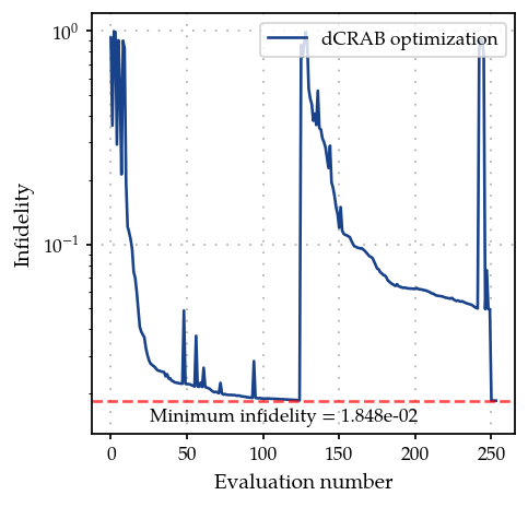
{'status': 2, 'value': 0.01848404858601005, 'iterations': 129, 'message': 'callback raised StopIteration.'}
Lets set the optimization to the best parameters obtained during the run
opt.set_parameters(opt.best_params)
[Amplitude CRAB resonator: 4.71e+07,
 CRAB Re coefficient 0: 0.638,
 CRAB Re coefficient 1: -0.752,
 CRAB Re coefficient 2: 0,
 CRAB Re coefficient 3: 0,
 CRAB Re coefficient 4: 0,
 CRAB Re coefficient 5: 0,
 CRAB Re frequency 0: 1.34 Hz x 2pi,
 CRAB Re frequency 1: 763 mHz x 2pi,
 CRAB Re frequency 2: 1 Hz x 2pi,
 CRAB Re frequency 3: 1 Hz x 2pi,
 CRAB Re frequency 4: 1 Hz x 2pi,
 CRAB Re frequency 5: 1 Hz x 2pi,
 CRAB Re Phase 0: 70.6 mHz x 2pi,
 CRAB Re Phase 1: -318 mHz x 2pi,
 CRAB Re Phase 2: 0 Hz x 2pi,
 CRAB Re Phase 3: 0 Hz x 2pi,
 CRAB Re Phase 4: 0 Hz x 2pi,
 CRAB Re Phase 5: 0 Hz x 2pi,
 CRAB Im coefficient 0: -0.418,
 CRAB Im coefficient 1: 0.941,
 CRAB Im coefficient 2: 0,
 CRAB Im coefficient 3: 0,
 CRAB Im coefficient 4: 0,
 CRAB Im coefficient 5: 0,
 CRAB Im frequency 0: 1.7 Hz x 2pi,
 CRAB Im frequency 1: 1.88 Hz x 2pi,
 CRAB Im frequency 2: 1 Hz x 2pi,
 CRAB Im frequency 3: 1 Hz x 2pi,
 CRAB Im frequency 4: 1 Hz x 2pi,
 CRAB Im frequency 5: 1 Hz x 2pi,
 CRAB Im Phase 0: -89.7 mHz x 2pi,
 CRAB Im Phase 1: 500 mHz x 2pi,
 CRAB Im phase 2: 0 Hz x 2pi,
 CRAB Im phase 3: 0 Hz x 2pi,
 CRAB Im phase 4: 0 Hz x 2pi,
 CRAB Im phase 5: 0 Hz x 2pi,
 Amplitude CRAB qubit: -4.32e+07,
 CRAB Re coefficient 0: 0.819,
 CRAB Re coefficient 1: -0.809,
 CRAB Re coefficient 2: 0,
 CRAB Re coefficient 3: 0,
 CRAB Re coefficient 4: 0,
 CRAB Re coefficient 5: 0,
 CRAB Re frequency 0: 1.68 Hz x 2pi,
 CRAB Re frequency 1: 995 mHz x 2pi,
 CRAB Re frequency 2: 1 Hz x 2pi,
 CRAB Re frequency 3: 1 Hz x 2pi,
 CRAB Re frequency 4: 1 Hz x 2pi,
 CRAB Re frequency 5: 1 Hz x 2pi,
 CRAB Re Phase 0: 386 mHz x 2pi,
 CRAB Re Phase 1: 473 mHz x 2pi,
 CRAB Re Phase 2: 0 Hz x 2pi,
 CRAB Re Phase 3: 0 Hz x 2pi,
 CRAB Re Phase 4: 0 Hz x 2pi,
 CRAB Re Phase 5: 0 Hz x 2pi,
 CRAB Im coefficient 0: 0.541,
 CRAB Im coefficient 1: -0.395,
 CRAB Im coefficient 2: 0,
 CRAB Im coefficient 3: 0,
 CRAB Im coefficient 4: 0,
 CRAB Im coefficient 5: 0,
 CRAB Im frequency 0: 1.86 Hz x 2pi,
 CRAB Im frequency 1: 702 mHz x 2pi,
 CRAB Im frequency 2: 1 Hz x 2pi,
 CRAB Im frequency 3: 1 Hz x 2pi,
 CRAB Im frequency 4: 1 Hz x 2pi,
 CRAB Im frequency 5: 1 Hz x 2pi,
 CRAB Im Phase 0: 155 mHz x 2pi,
 CRAB Im Phase 1: -12.5 mHz x 2pi,
 CRAB Im phase 2: 0 Hz x 2pi,
 CRAB Im phase 3: 0 Hz x 2pi,
 CRAB Im phase 4: 0 Hz x 2pi,
 CRAB Im phase 5: 0 Hz x 2pi]
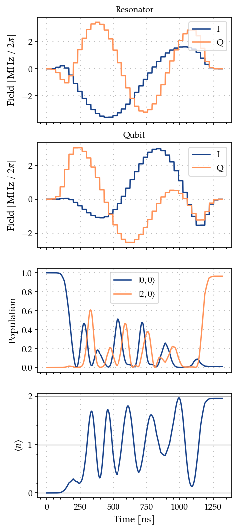
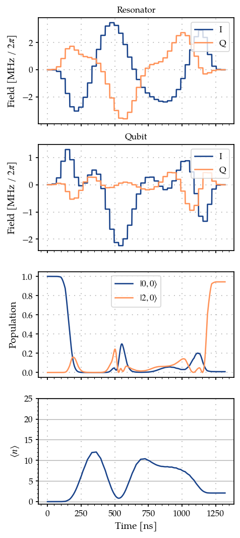
We can now plot the new pulses and the corresponding dynamics. If the number of iterations (max_iter) is chosen to be large enough, we should see an improvement.
plot_states_and_fock_number()
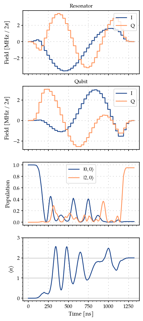
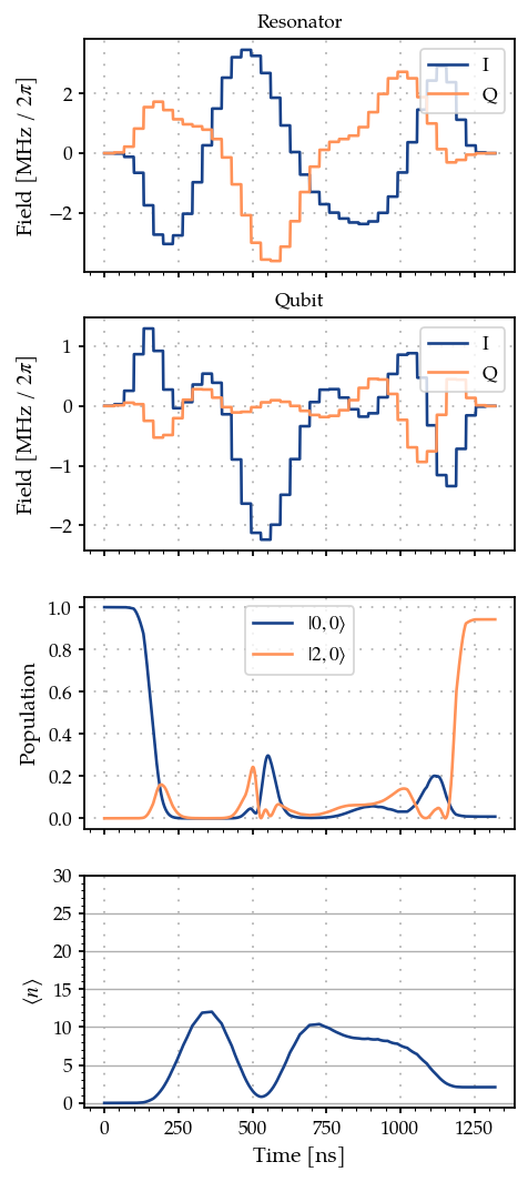
We can also compare the dynamics with the higher truncation number. Ideally, if the pulse amplitude is not high enough to produce artifacts due to the truncation of Hilbert space, the dyanmics in the two cases should match each other. Else one needs to either reduce the pulse amplitude or increase the truncation cutoff.
plot_states_and_fock_number(1)
The new fidelities are
print(f"Fidelity at N_T={n_fock_truncation_list[0]} = {dcrab_meas_list[0].measure()}")
print(f"Fidelity at N_T={n_fock_truncation_list[1]} = {dcrab_meas_list[1].measure()}")
Fidelity at N_T=3 = 0.9644227153981635
Fidelity at N_T=4 = 0.9495444579862979
For this small truncation number the dynamics and fidelities do not match very well. This indicates the need for higher truncation numbers, which we demonstrate in the next section.
Finally, lets plot the variation of infidelity with evaluation number.
from plotting import plot_infidelity_vs_evaluation_from_logs

plot_infidelity_vs_evaluation_from_logs(log_path=temp_dir.name + "/opt.log", label="dCRAB optimization");
Setting trunction to higher value
Here we set the truncation values to 30 and 31 levels for a more realistic simualtion and rerun the entire simulation.
Note - The following takes about 60 mins to run on an AMD-EPYC Milan processor with 128 cores and 256GB RAM (might take more depending on the number of CPU cores available).
We first reset the generator parameters (by redefining them), and redefine the resonator with higher truncation numbers.
# in seconds (See Eickbusch et al https://arxiv.org/abs/2111.06414 S9 A)
delta_sampling = 33e-9
n_pwc = 40  # number of piecewise constants in the pulse
t_final = n_pwc * delta_sampling  # for now just set up for trying
tlist = np.linspace(0, t_final, n_pwc + 1)
eps_res = 3 * np.pi * 1.0  # initial amplitude of the resonator (in MHz)
eps_max_res = 5 * eps_res  # maximum amplitude of the resonator (in MHz)
eps_qubit = 3 * np.pi * 1.0  # initial amplitude of the qubit (in MHz)
eps_max_qubit = 5 * eps_qubit  # maximum amplitude of the resonator (in MHz)

tone_res = DCRABEnvelope(
    num_components=3,
    max_frequency=2 * np.pi * 5.0,
    amplitude=Quantity(eps_res * 1e6, -eps_max_res * 1e6, eps_max_res * 1e6, name="Amplitude CRAB resonator"),
    t_final=Quantity(t_final, 1 / 2 * t_final, 2 * t_final, name="t_final CRAB resonator"),
    seed=17619276394480986,
)

smooth_tone_res = FlatTopGaussianFilter(
    envelopes=tone_res, t_final=Quantity(t_final, 1 / 2 * t_final, 2 * t_final, name="t_final")
)

tone_qubit = DCRABEnvelope(
    num_components=3,
    max_frequency=2 * np.pi * 5.0,
    amplitude=Quantity(eps_qubit * 1e6, -eps_max_qubit * 1e6, eps_max_qubit * 1e6, name="Amplitude CRAB qubit"),
    t_final=Quantity(t_final, 1 / 2 * t_final, 2 * t_final, name="t_final CRAB qubit"),
    seed=17619276394849436,
)

smooth_tone_qubit = FlatTopGaussianFilter(
    envelopes=tone_qubit, t_final=Quantity(t_final, 1 / 2 * t_final, 2 * t_final, name="t_final")
)

gen_res = PWCGenerator(envelopes=[smooth_tone_res], tlist=tlist, max_amplitude=2 * eps_max_res * 1e6)
gen_qubit = PWCGenerator(envelopes=[smooth_tone_qubit], tlist=tlist, max_amplitude=2 * eps_max_qubit * 71e6)
# Increasing the number of Fock states gives a more realistic scenario, at the price of increasing the simulation time
n_fock_truncation_list = [30, 31]
fock_target = 2
n_times = 1001

omega_range_factor = 1e-3  # just for initialization of the Quantity object
omega_res = 2 * np.pi * 5.26e9
omega_qubit = 2 * np.pi * 6.65e9

omega_drive_res = omega_res
omega_drive_qubit = omega_qubit

detuning_drive_res = omega_res - omega_drive_res
detuning_drive_qubit = omega_qubit - omega_drive_qubit

drive_res = RotatingFrameDrive(gen_res)
drive_qubit = RotatingFrameDrive(gen_qubit)


# Create a new experiment and redefine the measurement
initial_state_list, target_state_list, fock_number_op_list, prop_list, dcrab_meas_list = create_experiment(
    n_fock_truncation_list, fock_target
)

weights = np.array([1.0 for _ in range(len(dcrab_meas_list))])
weight_sum_of_squares = -0.05
total_sum_of_weights = np.sum(weights) + weight_sum_of_squares
weights = weights / total_sum_of_weights
weight_sum_of_squares = weight_sum_of_squares / total_sum_of_weights
dcrab_meas_list_bool = [True for meas in dcrab_meas_list]
sum_of_squares_options = {"weight": weight_sum_of_squares, "meas_bool": dcrab_meas_list_bool}

dcrab_goal = WeightedSumGoal(dcrab_meas_list, weights, sum_of_squares_options=sum_of_squares_options)
plot_states_and_fock_number()
plot_states_and_fock_number(1)

Initial fidelity before optimization
print(f"Fidelity at N_T={n_fock_truncation_list[0]} = {dcrab_meas_list[0].measure()}")
print(f"Fidelity at N_T={n_fock_truncation_list[1]} = {dcrab_meas_list[1].measure()}")
Fidelity at N_T=30 = 0.00809359027771987
Fidelity at N_T=31 = 0.00809359027771987
tone_res.get_parameters()
[Amplitude CRAB resonator: 9.42e+06,
 t_final CRAB resonator: 1.32e-06,
 CRAB Re coefficient 0: -0.218,
 CRAB Re coefficient 1: -0.711,
 CRAB Re coefficient 2: -0.223,
 CRAB Re frequency 0: 4.77 Hz x 2pi,
 CRAB Re frequency 1: 4.34 Hz x 2pi,
 CRAB Re frequency 2: 4.59 Hz x 2pi,
 CRAB Re Phase 0: 478 mHz x 2pi,
 CRAB Re Phase 1: 5.23 mHz x 2pi,
 CRAB Re Phase 2: 415 mHz x 2pi,
 CRAB Im coefficient 0: -0.725,
 CRAB Im coefficient 1: -0.262,
 CRAB Im coefficient 2: 0.901,
 CRAB Im frequency 0: 3.33 Hz x 2pi,
 CRAB Im frequency 1: 3.18 Hz x 2pi,
 CRAB Im frequency 2: 1.97 Hz x 2pi,
 CRAB Im Phase 0: 205 mHz x 2pi,
 CRAB Im Phase 1: 230 mHz x 2pi,
 CRAB Im Phase 2: 60.2 mHz x 2pi]
tone_qubit.get_parameters()
[Amplitude CRAB qubit: 9.42e+06,
 t_final CRAB qubit: 1.32e-06,
 CRAB Re coefficient 0: -0.693,
 CRAB Re coefficient 1: 0.833,
 CRAB Re coefficient 2: 0.687,
 CRAB Re frequency 0: 4.03 Hz x 2pi,
 CRAB Re frequency 1: 2.46 Hz x 2pi,
 CRAB Re frequency 2: 4.43 Hz x 2pi,
 CRAB Re Phase 0: -98.2 mHz x 2pi,
 CRAB Re Phase 1: -341 mHz x 2pi,
 CRAB Re Phase 2: -211 mHz x 2pi,
 CRAB Im coefficient 0: -0.152,
 CRAB Im coefficient 1: -0.103,
 CRAB Im coefficient 2: 0.579,
 CRAB Im frequency 0: 2.09 Hz x 2pi,
 CRAB Im frequency 1: 4.5 Hz x 2pi,
 CRAB Im frequency 2: 2.08 Hz x 2pi,
 CRAB Im Phase 0: -353 mHz x 2pi,
 CRAB Im Phase 1: 481 mHz x 2pi,
 CRAB Im Phase 2: -16.3 mHz x 2pi]
Redefine the optmap and the optmizer and rerun the optimization
import tempfile

temp_dir = tempfile.TemporaryDirectory()
print(f"Logging directory = {temp_dir.name}")

max_iter = 1000  # set to 1000 for a good result; set to 10 for a quick example
optmap = OptimisationMap()
optmap.add(tone_res)
optmap.add(tone_qubit)

# Remove the t_final and  DRAG Delta from optimisation from drag tone resonator and qubit
optmap.remove(tone_qubit, params_tone_qubit[1])
optmap.remove(tone_res, params_tone_res[1])
optmap.register_params_with_optimisables()

file_logger = FileLogger(temp_dir.name)

# Define the optimiser
opt = DCRABOptimiserGradient(
    dcrab_goal,
    optimisation_map=optmap,
    super_iteration_every=500,
    max_super_iteration_num=3,
    print_every_iteration_num=10,
    super_iteration_tol=1e-6,
    seed=8647,
)
opt.set_options({"maxfun": max_iter, "workers": 32})
opt.logger = file_logger
Logging directory = /tmp/tmppoaajj37
Implicitly cleaning up <TemporaryDirectory '/tmp/tmp1qve13ga'>
opt.optimise()
opt.set_parameters(opt.best_params)
Iteration number = 0          Infidelity  = 9.040e-01
Iteration number = 10         Infidelity  = 7.051e-01
Iteration number = 20         Infidelity  = 6.287e-01
Iteration number = 30         Infidelity  = 5.699e-01
Iteration number = 40         Infidelity  = 5.296e-01
Iteration number = 50         Infidelity  = 5.090e-01


==== Decrease in infidelity less than 1e-06 ====
==== Starting super-iteration 1 ====
* Current lowest infidelity =  5.065e-01
* Current no. of parameters = 74
Iteration number = 60         Infidelity  = 7.309e-01
Iteration number = 70         Infidelity  = 6.711e-01
Iteration number = 80         Infidelity  = 5.943e-01
Iteration number = 90         Infidelity  = 5.457e-01
Iteration number = 100        Infidelity  = 5.092e-01
Iteration number = 110        Infidelity  = 4.889e-01
Iteration number = 120        Infidelity  = 4.637e-01
Iteration number = 130        Infidelity  = 4.350e-01
Iteration number = 140        Infidelity  = 4.204e-01
Iteration number = 150        Infidelity  = 4.048e-01
Iteration number = 160        Infidelity  = 3.780e-01
Iteration number = 170        Infidelity  = 3.578e-01
Iteration number = 180        Infidelity  = 3.425e-01
Iteration number = 190        Infidelity  = 3.312e-01
Iteration number = 200        Infidelity  = 3.212e-01
Iteration number = 210        Infidelity  = 3.125e-01
Iteration number = 220        Infidelity  = 3.087e-01
Iteration number = 230        Infidelity  = 3.053e-01
Iteration number = 240        Infidelity  = 3.000e-01
Iteration number = 250        Infidelity  = 2.947e-01
Iteration number = 260        Infidelity  = 2.914e-01
Iteration number = 270        Infidelity  = 2.901e-01
Iteration number = 280        Infidelity  = 2.883e-01
Iteration number = 290        Infidelity  = 2.869e-01
Iteration number = 300        Infidelity  = 2.853e-01
Iteration number = 310        Infidelity  = 2.838e-01
Iteration number = 320        Infidelity  = 2.810e-01
Iteration number = 330        Infidelity  = 2.780e-01
Iteration number = 340        Infidelity  = 2.747e-01
Iteration number = 350        Infidelity  = 2.726e-01
Iteration number = 360        Infidelity  = 2.692e-01
Iteration number = 370        Infidelity  = 2.676e-01
Iteration number = 380        Infidelity  = 2.656e-01
Iteration number = 390        Infidelity  = 2.638e-01
Iteration number = 400        Infidelity  = 2.612e-01
Iteration number = 410        Infidelity  = 2.596e-01
Iteration number = 420        Infidelity  = 2.583e-01
Iteration number = 430        Infidelity  = 2.576e-01
Iteration number = 440        Infidelity  = 2.570e-01
Iteration number = 450        Infidelity  = 2.560e-01
Iteration number = 460        Infidelity  = 2.550e-01
Iteration number = 470        Infidelity  = 2.548e-01


==== Decrease in infidelity less than 1e-06 ====
==== Starting super-iteration 2 ====
* Current lowest infidelity =  2.546e-01
* Current no. of parameters = 110
Iteration number = 480        Infidelity  = 5.692e-01
Iteration number = 490        Infidelity  = 3.303e-01
Iteration number = 500        Infidelity  = 2.757e-01
Iteration number = 510        Infidelity  = 2.579e-01
Iteration number = 520        Infidelity  = 2.504e-01
Iteration number = 530        Infidelity  = 2.460e-01
Iteration number = 540        Infidelity  = 2.377e-01
Iteration number = 550        Infidelity  = 2.321e-01
Iteration number = 560        Infidelity  = 2.226e-01
Iteration number = 570        Infidelity  = 2.158e-01
Iteration number = 580        Infidelity  = 2.081e-01
Iteration number = 590        Infidelity  = 1.983e-01
Iteration number = 600        Infidelity  = 1.909e-01
Iteration number = 610        Infidelity  = 1.865e-01
Iteration number = 620        Infidelity  = 1.815e-01
Iteration number = 630        Infidelity  = 1.761e-01
Iteration number = 640        Infidelity  = 1.737e-01
Iteration number = 650        Infidelity  = 1.683e-01
Iteration number = 660        Infidelity  = 1.655e-01
Iteration number = 670        Infidelity  = 1.630e-01
Iteration number = 680        Infidelity  = 1.616e-01
Iteration number = 690        Infidelity  = 1.605e-01
Iteration number = 700        Infidelity  = 1.594e-01
Iteration number = 710        Infidelity  = 1.586e-01
Iteration number = 720        Infidelity  = 1.578e-01
Iteration number = 730        Infidelity  = 1.573e-01
Iteration number = 740        Infidelity  = 1.564e-01
Iteration number = 750        Infidelity  = 1.552e-01
Iteration number = 760        Infidelity  = 1.534e-01
Iteration number = 770        Infidelity  = 1.522e-01
Iteration number = 780        Infidelity  = 1.507e-01
Iteration number = 790        Infidelity  = 1.484e-01
Iteration number = 800        Infidelity  = 1.461e-01
Iteration number = 810        Infidelity  = 1.451e-01
Iteration number = 820        Infidelity  = 1.441e-01
Iteration number = 830        Infidelity  = 1.421e-01
Iteration number = 840        Infidelity  = 1.381e-01
Iteration number = 850        Infidelity  = 1.279e-01
Iteration number = 860        Infidelity  = 1.138e-01
Iteration number = 870        Infidelity  = 1.010e-01
Iteration number = 880        Infidelity  = 8.504e-02
Iteration number = 890        Infidelity  = 7.778e-02
Iteration number = 900        Infidelity  = 6.981e-02
Iteration number = 910        Infidelity  = 6.408e-02
Iteration number = 920        Infidelity  = 5.855e-02
Iteration number = 930        Infidelity  = 5.534e-02
Iteration number = 940        Infidelity  = 5.077e-02
Iteration number = 950        Infidelity  = 4.271e-02
Iteration number = 960        Infidelity  = 3.868e-02
Iteration number = 970        Infidelity  = 3.561e-02


==== Max iteration before a super-iteration reached ====
==== Starting super-iteration 3 ====
* Current lowest infidelity =  0.033 *
* Current no. of parameters = 146
Stopping the optimisation or backtracking to previous best fidelity. Going to step with 110 parameters.
Stopping the optimisation or backtracking to previous best fidelity. Going to step with 74 parameters.
Iteration number = 980 Infidelity = 2.546e-01
Stopping the optimisation or backtracking to previous best fidelity. Going to step with 38 parameters.
Setting parameters to the best values.
[Amplitude CRAB resonator: 4.71e+07,
 CRAB Re coefficient 0: 0.00911,
 CRAB Re coefficient 1: -0.172,
 CRAB Re coefficient 2: -0.0199,
 CRAB Re coefficient 3: -0.00569,
 CRAB Re coefficient 4: -1,
 CRAB Re coefficient 5: 0.0037,
 CRAB Re coefficient 6: 0.253,
 CRAB Re coefficient 7: -0.904,
 CRAB Re coefficient 8: -0.234,
 CRAB Re coefficient 9: 0,
 CRAB Re coefficient 10: 0,
 CRAB Re coefficient 11: 0,
 CRAB Re frequency 0: 4.81 Hz x 2pi,
 CRAB Re frequency 1: 2.42 Hz x 2pi,
 CRAB Re frequency 2: 4.71 Hz x 2pi,
 CRAB Re frequency 3: 4.75 Hz x 2pi,
 CRAB Re frequency 4: 1.93 Hz x 2pi,
 CRAB Re frequency 5: 4.69 Hz x 2pi,
 CRAB Re frequency 6: 3.6 Hz x 2pi,
 CRAB Re frequency 7: 1.94 Hz x 2pi,
 CRAB Re frequency 8: 3.47 Hz x 2pi,
 CRAB Re frequency 9: 2.5 Hz x 2pi,
 CRAB Re frequency 10: 2.5 Hz x 2pi,
 CRAB Re frequency 11: 2.5 Hz x 2pi,
 CRAB Re Phase 0: 499 mHz x 2pi,
 CRAB Re Phase 1: 500 mHz x 2pi,
 CRAB Re Phase 2: 498 mHz x 2pi,
 CRAB Re Phase 3: 491 mHz x 2pi,
 CRAB Re Phase 4: -222 mHz x 2pi,
 CRAB Re Phase 5: -442 mHz x 2pi,
 CRAB Re Phase 6: -213 mHz x 2pi,
 CRAB Re Phase 7: -238 mHz x 2pi,
 CRAB Re Phase 8: 333 mHz x 2pi,
 CRAB Re Phase 9: 0 Hz x 2pi,
 CRAB Re Phase 10: 0 Hz x 2pi,
 CRAB Re Phase 11: 0 Hz x 2pi,
 CRAB Im coefficient 0: -0.0288,
 CRAB Im coefficient 1: -0.415,
 CRAB Im coefficient 2: -0.0142,
 CRAB Im coefficient 3: 0.00796,
 CRAB Im coefficient 4: -0.55,
 CRAB Im coefficient 5: -0.985,
 CRAB Im coefficient 6: -0.000222,
 CRAB Im coefficient 7: 0.0207,
 CRAB Im coefficient 8: 0.0198,
 CRAB Im coefficient 9: 0,
 CRAB Im coefficient 10: 0,
 CRAB Im coefficient 11: 0,
 CRAB Im frequency 0: 3.07 Hz x 2pi,
 CRAB Im frequency 1: 4.18 Hz x 2pi,
 CRAB Im frequency 2: 4.95 Hz x 2pi,
 CRAB Im frequency 3: 4.97 Hz x 2pi,
 CRAB Im frequency 4: 2.12 Hz x 2pi,
 CRAB Im frequency 5: 1.36 Hz x 2pi,
 CRAB Im frequency 6: 4 Hz x 2pi,
 CRAB Im frequency 7: 4.97 Hz x 2pi,
 CRAB Im frequency 8: 3.94 Hz x 2pi,
 CRAB Im frequency 9: 2.5 Hz x 2pi,
 CRAB Im frequency 10: 2.5 Hz x 2pi,
 CRAB Im frequency 11: 2.5 Hz x 2pi,
 CRAB Im Phase 0: 500 mHz x 2pi,
 CRAB Im Phase 1: 241 mHz x 2pi,
 CRAB Im Phase 2: -187 mHz x 2pi,
 CRAB Im phase 3: 342 mHz x 2pi,
 CRAB Im phase 4: 92.6 mHz x 2pi,
 CRAB Im phase 5: 411 mHz x 2pi,
 CRAB Im phase 6: -6.39 mHz x 2pi,
 CRAB Im phase 7: 130 mHz x 2pi,
 CRAB Im phase 8: -66 mHz x 2pi,
 CRAB Im phase 9: 0 Hz x 2pi,
 CRAB Im phase 10: 0 Hz x 2pi,
 CRAB Im phase 11: 0 Hz x 2pi,
 Amplitude CRAB qubit: 4.36e+07,
 CRAB Re coefficient 0: -0.433,
 CRAB Re coefficient 1: 0.0102,
 CRAB Re coefficient 2: 0.0482,
 CRAB Re coefficient 3: -0.742,
 CRAB Re coefficient 4: -0.0313,
 CRAB Re coefficient 5: 0.188,
 CRAB Re coefficient 6: 0.974,
 CRAB Re coefficient 7: -0.133,
 CRAB Re coefficient 8: -0.458,
 CRAB Re coefficient 9: 0,
 CRAB Re coefficient 10: 0,
 CRAB Re coefficient 11: 0,
 CRAB Re frequency 0: 5 Hz x 2pi,
 CRAB Re frequency 1: 3.33 Hz x 2pi,
 CRAB Re frequency 2: 4.4 Hz x 2pi,
 CRAB Re frequency 3: 4.29 Hz x 2pi,
 CRAB Re frequency 4: 3.57 Hz x 2pi,
 CRAB Re frequency 5: 4.51 Hz x 2pi,
 CRAB Re frequency 6: 1.82 Hz x 2pi,
 CRAB Re frequency 7: 1.12 Hz x 2pi,
 CRAB Re frequency 8: 738 mHz x 2pi,
 CRAB Re frequency 9: 2.5 Hz x 2pi,
 CRAB Re frequency 10: 2.5 Hz x 2pi,
 CRAB Re frequency 11: 2.5 Hz x 2pi,
 CRAB Re Phase 0: 289 mHz x 2pi,
 CRAB Re Phase 1: -386 mHz x 2pi,
 CRAB Re Phase 2: -419 mHz x 2pi,
 CRAB Re Phase 3: 195 mHz x 2pi,
 CRAB Re Phase 4: -185 mHz x 2pi,
 CRAB Re Phase 5: 498 mHz x 2pi,
 CRAB Re Phase 6: -209 mHz x 2pi,
 CRAB Re Phase 7: 412 mHz x 2pi,
 CRAB Re Phase 8: -436 mHz x 2pi,
 CRAB Re Phase 9: 0 Hz x 2pi,
 CRAB Re Phase 10: 0 Hz x 2pi,
 CRAB Re Phase 11: 0 Hz x 2pi,
 CRAB Im coefficient 0: -0.529,
 CRAB Im coefficient 1: -0.237,
 CRAB Im coefficient 2: 0.717,
 CRAB Im coefficient 3: 0.446,
 CRAB Im coefficient 4: -0.648,
 CRAB Im coefficient 5: 0.418,
 CRAB Im coefficient 6: 0.672,
 CRAB Im coefficient 7: -0.136,
 CRAB Im coefficient 8: -0.199,
 CRAB Im coefficient 9: 0,
 CRAB Im coefficient 10: 0,
 CRAB Im coefficient 11: 0,
 CRAB Im frequency 0: 4.28 Hz x 2pi,
 CRAB Im frequency 1: 5 Hz x 2pi,
 CRAB Im frequency 2: 4.56 Hz x 2pi,
 CRAB Im frequency 3: 4.89 Hz x 2pi,
 CRAB Im frequency 4: 5 Hz x 2pi,
 CRAB Im frequency 5: 3.8 Hz x 2pi,
 CRAB Im frequency 6: 4.62 Hz x 2pi,
 CRAB Im frequency 7: 3.72 Hz x 2pi,
 CRAB Im frequency 8: 4.32 Hz x 2pi,
 CRAB Im frequency 9: 2.5 Hz x 2pi,
 CRAB Im frequency 10: 2.5 Hz x 2pi,
 CRAB Im frequency 11: 2.5 Hz x 2pi,
 CRAB Im Phase 0: -329 mHz x 2pi,
 CRAB Im Phase 1: 500 mHz x 2pi,
 CRAB Im Phase 2: -225 mHz x 2pi,
 CRAB Im phase 3: 388 mHz x 2pi,
 CRAB Im phase 4: 500 mHz x 2pi,
 CRAB Im phase 5: -292 mHz x 2pi,
 CRAB Im phase 6: -317 mHz x 2pi,
 CRAB Im phase 7: 226 mHz x 2pi,
 CRAB Im phase 8: -323 mHz x 2pi,
 CRAB Im phase 9: 0 Hz x 2pi,
 CRAB Im phase 10: 0 Hz x 2pi,
 CRAB Im phase 11: 0 Hz x 2pi]
And the new fidelities are
print(f"Fidelity at N_T={n_fock_truncation_list[0]} = {dcrab_meas_list[0].measure()}")
print(f"Fidelity at N_T={n_fock_truncation_list[1]} = {dcrab_meas_list[1].measure()}")
Fidelity at N_T=30 = 0.9430470710184967
Fidelity at N_T=31 = 0.9422620192354791
Here the dynamics and the fidelities are very similar to one another, indicating no truncation artifacts.
Lets plot the optimised pulses and dyanmics
plot_states_and_fock_number()
And verify the dynamics with the higher truncation looks the same
plot_states_and_fock_number(1)
Finally, lets plot the variation of infidelity with evaluation number.
from plotting import plot_infidelity_vs_evaluation_from_logs

plot_infidelity_vs_evaluation_from_logs(log_path=temp_dir.name + "/opt.log", label="dCRAB optimization");
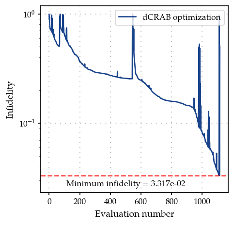
The sharp rise infidelity represents the beginning of a super-iteration