State transfer control of a single spin

First, we make the necessary imports.

import numpy as np

from paraqeet.optimisation_map import OptimisationMap
from paraqeet.quantity import Quantity
from paraqeet.measurement.state_transfer_fidelity import StateTransferFidelity
from paraqeet.model.drive_operator import DriveOperator
from paraqeet.model.qubit import Qubit
from paraqeet.propagation.scipy_expm import ScipyExpm
from paraqeet.optimisers.scipy_optimiser import ScipyOptimiser

from paraqeet.model.closed_system import ClosedSystem

from paraqeet.signal.iq_mixer import IQMixer
from paraqeet.signal.envelopes import ConstantEnvelope

System Setup

For signal generation, we define a simple cosine shaped tone generator \(A \cos(\omega t)\)

tone = ConstantEnvelope()
gen = IQMixer(envelopes=[tone])

We can inspect the pre-defined parameters with

params = gen.get_parameters()
params

[Amplitude: 24.7 MHz x 2pi,
 t_final: 32 ns,
 lo_freq: 4.8 GHz x 2pi,
 Phase: 0 rad]

in this case amplitude \(A\) and frequency \(\omega\).

Next, we setup the qubit system we want to control. We set the qubit frequency \(\omega_q\) to be 4.8 GHz and define the Hamiltonian as

\[H(t)=H_\text{drift}+H_c(t)= \frac{\omega_q}{2} \sigma_z + \Omega(t)\sigma_x\]

, where \(\Omega(t)\) will be supplied by the generator.

freq = 4.8e9 * 2 * np.pi

drive = DriveOperator(gen, is_longitudinal=False)
controlled_qubit = Qubit(frequency=Quantity(freq, 0.8 * freq, 1.2 * freq), drives=[drive])
model = ClosedSystem(controlled_qubit)

Textbook values for implementing an \(X\) rotation on this system at a time \(T\) would be \(\omega=\omega_q\) and \(A=\pi/T\). We use some offset from these values as initial guess to demonstrate the optimization procedure.

t_final = 10e-9
params[0].set_value(0.8 * np.pi / t_final)
params[2].set_value(1.01 * freq)

We select a propagation method, piecewise constant exponentation, and configure a state transfer problem from \(\ket{0}\) to \(\ket{1}\).

prop = ScipyExpm(model, res=100e9)

init = np.array([[1.0], [0]])  # |0>
target = np.array([[0.0], [1]])  # |1>
zeroone = StateTransferFidelity(
    propagation=prop,
    initial_state=init,
    target_state=target,
    times=np.array([0.0, t_final]),
)

Population dynamics

from plotting import plot_signal_and_dynamics

ts = np.linspace(0.0, t_final, 101)
plot_signal_and_dynamics(gen, prop, ts, state_labels=[r"$|0\rangle$", r"$|1\rangle$"]);

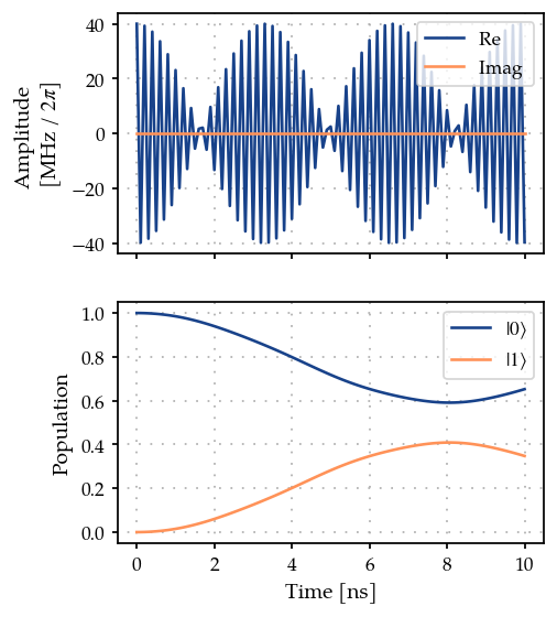
As expected, we get a partial transfer and a low fidelity.

zeroone.measure()

0.34736071270511687

Optimisation

We define an optimizer and link our fidelity measure as a goal function and the parameters of the cosine tone.

optmap = OptimisationMap()
optmap.add(tone, params)
opt = ScipyOptimiser(zeroone, optimisation_map=optmap)

opt.optimise()

{'status': 1, 'value': 4.3098857815948577e-13, 'iterations': 55, 'message': 'CONVERGENCE: NORM OF PROJECTED GRADIENT <= PGTOL'}

plot_signal_and_dynamics(gen, prop, ts, state_labels=[r"$|0\rangle$", r"$|1\rangle$"]);

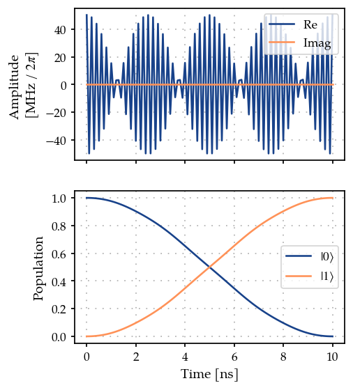
We can see from the plot and optimizer output that we have found good controls.

zeroone.measure()

0.9999999999995541

params

[Amplitude: 50.2 MHz x 2pi,
 t_final: 32 ns,
 lo_freq: 4.8 GHz x 2pi,
 Phase: 615 µrad]

and parameters close to the textbook values:

np.pi / t_final, freq

(314159265.3589793, 30159289474.462013)