Optimal control of a single spin by using GOAT over GRAPE

In this introductory example we compute the gradients of analytic pulse shapes in GOAT by using the gradients of the time evolition from GRAPE. This is performed by using chain rule -

\[\frac{\partial J}{\partial p} = \sum_k \frac{\partial J}{\partial c_k} \frac{\partial c_k}{\partial p}\]

where \(c_k = c(t_k)\) the ‘pixelated’ control pulse, \(\vec{p}\) are the analytical parameters of the control pulse $c(t) :raw-latex:`\equiv `c(:raw-latex:`vec{p}`, t) $, and \(\frac{\partial J}{\partial c_k}\) are the gradients from GRAPE.

1. Generate a PWC pulse shape

import matplotlib.pyplot as plt
import numpy as np
from paraqeet.quantity import Quantity

from paraqeet.signal.pwc_generator import PWCGenerator

Lets define a FlatTopGaussianEnvelope with multiple optimisable parameters to check if the optimisation of all the parameters works when we rebuild them with GRAPE propagation. We can rely on Automatic differentiation to obtain the gradient of the pulse wrt its parameters.

from collections.abc import Callable
from functools import partial

from paraqeet.quantity import Array
import jax.numpy as jnp

from jax import jit
from jax.scipy.special import erf
from paraqeet.signal.envelopes import Envelope
from paraqeet.signal.waveform import FlatTopGaussianFilter


class FlatTopGaussianEnvelope(Envelope):
    """A flat-top Gaussian envelope."""

    def __init__(
        self,
        amplitude: Quantity,
        t_up: Quantity,
        t_down: Quantity,
        ramp_time: Quantity,
    ):
        self._amplitude = amplitude
        self.__t_up = t_up
        self.__t_down = t_down
        self.__ramp_time = ramp_time

        self._gradient_function: Callable | None = None
        self._grad_arg_nums: tuple[int, ...] = ()

    def get_parameters(self):
        """Get all parameters of the system."""
        return [self._amplitude, self.__t_up, self.__t_down, self.__ramp_time]

    @partial(jit, static_argnums=(0,))
    def _evaluate(self, amp: Array, t_up: Array, t_down: Array, ramp_time: Array, t: Array):
        ramp_up = 1 + erf((t - t_up) / ramp_time)
        ramp_down = 1 + erf((-t + t_down) / ramp_time)
        return jnp.squeeze(amp * ramp_up * ramp_down / 4)

    def compute_output(self, t: Array) -> Array:
        """Compute pulse shape."""
        amp = self._amplitude.get_value()
        t_up = self.__t_up.get_value()
        t_down = self.__t_down.get_value()
        ramp_time = self.__ramp_time.get_value()
        return self._evaluate(amp, t_up, t_down, ramp_time, t)

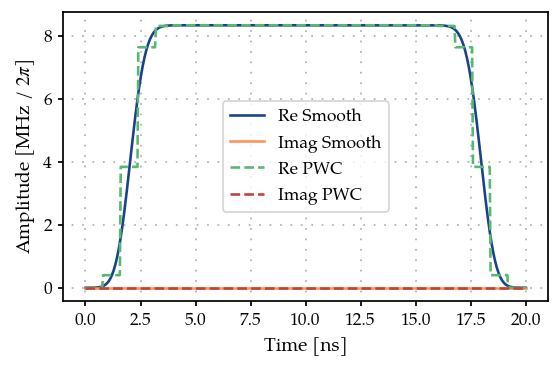
Define the Envelope and the PWCGenerator. The PWCGenerator is used to produce the pixelated pulse shape for computing the gradients using GRAPE. The optimisation would be performed on the Envelope parameters: amplitude, t_up, t_down, ramp_time.

t_final = 20e-9
tlist = np.linspace(0, t_final, 26)

tone = FlatTopGaussianEnvelope(
    amplitude=Quantity(np.pi / t_final / 3, -np.pi / t_final, np.pi / t_final, name="Amplitude"),
    t_up=Quantity(1e-9, 0.0, t_final, name="t_up"),
    t_down=Quantity(t_final - 1e-9, 0.0, t_final, name="t_down"),
    ramp_time=Quantity(1e-9, 0.5e-9, t_final, name="ramp_time"),
)

tone_smooth = FlatTopGaussianFilter(tone, t_final=Quantity(t_final, 0.0, 1.2 * t_final, name="t_final"))

gen = PWCGenerator(envelopes=[tone_smooth], tlist=tlist)

params = gen.get_parameters()
params[0].set_limits(-200e6, 200e6)
params[1].set_limits(-200e6, 200e6)

from plotting import plot_signal

ts = np.linspace(0, t_final, 501)
fig, ax = plt.subplots(1, figsize=(5, 3))

plot_signal(tone_smooth, ts, ax, linestyle="-", label="Smooth")
plot_signal(gen, ts, ax, linestyle="--", label="PWC");

2. Define Hamiltonian in the rotating frame of drive

As a simple toy model, we use a single spin.

from paraqeet.model.closed_system import ClosedSystem
from paraqeet.model.rotating_frame_drive import RotatingFrameDrive
from paraqeet.model.hamiltonian import Hamiltonian


class SpinRWA(Hamiltonian):
    """A Single Spin."""

    def __init__(self, drives=None):
        super().__init__(drives)
        self.sigma_p = np.array([[0j, 1], [0, 0]])
        self.dim = 2

    def get_matrix_one_time(self, t):
        """Just sigma-X."""
        return self._drives[0].get_matrix_one_time(self.sigma_p, t)

    def gradient(self, t):
        """Gradient is just the drive matrix."""
        return self._drives[0].gradient(self.sigma_p, t)


drive = RotatingFrameDrive(gen)
spin = SpinRWA(drives=[drive])
model = ClosedSystem(spin)

Using GRAPE as the method to propagate and compute the gradients

from paraqeet.measurement.state_transfer_fidelity import StateTransferFidelityGRAPE
from paraqeet.propagation.scipy_expm_grape import ScipyExpmGRAPE


prop = ScipyExpmGRAPE(model, res=1e9)

init = np.array([[1.0], [0]])  # |0>
target = np.array([[0.0], [1]])  # |1>

prop.set_initial_state(init)
prop.target_state = target

zeroone = StateTransferFidelityGRAPE(
    propagation=prop,
    initial_state=init,
    target_state=target,
    times=tlist,
)

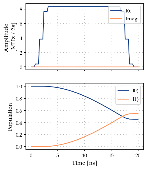
from plotting import plot_signal_and_dynamics

ts = np.linspace(0.0, t_final, 101)
plot_signal_and_dynamics(gen, prop, ts, state_labels=[r"$|0\rangle$", r"$|1\rangle$"]);

3. Optimisation

Finally, we define the GOATOverGRAPE fideltiy that chains together the GRAPE gradients to compute the gradient wrt the tone parameters

from paraqeet.optimisation_map import OptimisationMap
from paraqeet.optimisers.scipy_optimiser_gradient import ScipyOptimiserGradient
from paraqeet.measurement.goat_over_grape import GOATOverGRAPE

optmap = OptimisationMap()
optmap.add(tone)
optmap.register_params_with_optimisables()

goat = GOATOverGRAPE(zeroone, generators=[gen], generators_order=[0])
opt_grad = ScipyOptimiserGradient(goat, optimisation_map=optmap)

goat.measure_with_gradient()

(0.5458511041978135,
 Array([ 7.90501289e-09, -3.51099110e+06,  3.51099110e+06, -6.26131879e+06],      dtype=float64))

optmap.get_all_parameters()

[Amplitude: 5.24e+07, t_up: 1e-09, t_down: 1.9e-08, ramp_time: 1e-09]

optmap

==== <class '__main__.FlatTopGaussianEnvelope'> ====
[Amplitude: 5.24e+07, t_up: 1e-09, t_down: 1.9e-08, ramp_time: 1e-09]

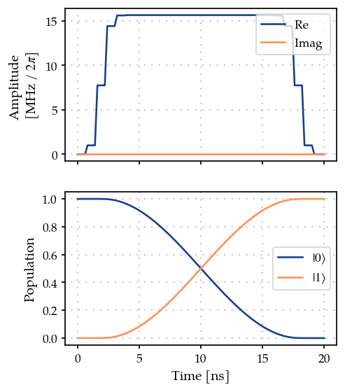
opt_grad.optimise()

{'status': 1, 'value': 2.220446049250313e-16, 'iterations': 6, 'message': 'CONVERGENCE: NORM OF PROJECTED GRADIENT <= PGTOL'}

For this simple example, we reach near perfect fidelity within a few iterations.

plot_signal_and_dynamics(gen, prop, ts, state_labels=[r"$|0\rangle$", r"$|1\rangle$"]);