Using a custom Hamiltonian function with ParaQeet

In this example we demonstrate how a custom Hamiltonian function H(t, params) can be used to simulate and optimise quantum systems.

import matplotlib.pyplot as plt
import jax.numpy as jnp
import paraqeet as pq

1. Define the parameters, Hamiltonian function and gradient functions

Define a Hamiltonian as a function of time and optimisable parameters. The optimisable paramter need to be of the type pq.Quantity.

Here we define a two level system (TLS) Hamiltonian, with a cosine drive (with optimisable paramters Amplitude and Frequency).

amplitude = pq.Quantity(
    value=jnp.array(1.55e8),
    min_value=jnp.array(0.0),
    max_value=jnp.array(5 * 1e8),
    unit="Hz",
    name="Amplitude",
    two_pi=True,
)

frequency = pq.Quantity(
    value=jnp.array(4.8e9 * 2 * jnp.pi),
    min_value=jnp.array(0.8 * 4.8e9 * 2 * jnp.pi),
    max_value=jnp.array(1.2 * 4.8e9 * 2 * jnp.pi),
    unit="Hz",
    name="lo_freq",
    two_pi=True,
)


def cos_envelope(t: pq.Array, amp, freq):
    """Define a cosine envelope."""
    return amp * jnp.cos(freq * t)


def tls_hamiltonian(t: pq.Array, amp, freq):
    """Define a Two level system Hamiltonian."""
    return 0.5 * freq * sigma_z + sigma_x * cos_envelope(t, amp, freq)


sigma_x = jnp.array([[0j, 1], [1, 0]])
sigma_z = jnp.diag(jnp.array([1.0, -1.0]))
freq = 4.8e9 * 2 * jnp.pi

from paraqeet.model.custom_hamiltonian import CustomHamiltonian
from paraqeet.model.closed_system import ClosedSystem

tls = CustomHamiltonian(
    hamiltonian_function=tls_hamiltonian,
    parameters=[amplitude, frequency],
)
model = ClosedSystem(tls)

2. Define propagation method and measurement function

Here we pick the standard ScipyExpmGOAT method for propagation and StateTransferFidelity as our measurement function

from paraqeet.measurement.state_transfer_fidelity import StateTransferFidelity
from paraqeet.propagation.scipy_expm_goat import ScipyExpmGOAT

t_final = 12e-9

prop = ScipyExpmGOAT(model, res=100e9)

init = jnp.array([[1.0], [0]])  # |0>
target = jnp.array([[0.0], [1]])  # |1>
zeroone = StateTransferFidelity(
    propagation=prop,
    initial_state=init,
    target_state=target,
    times=jnp.array([0.0, t_final]),
)

import plotting  # import the configuration from plotting


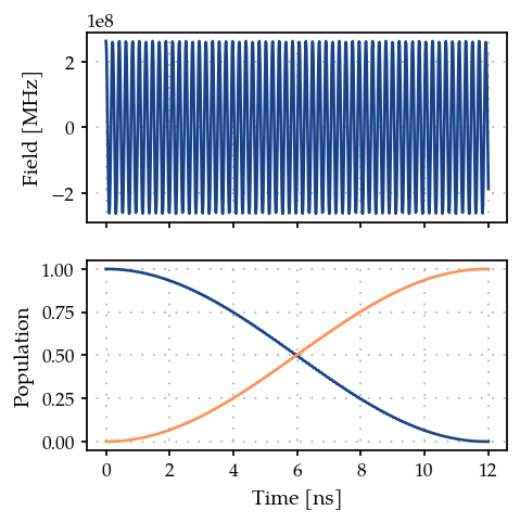
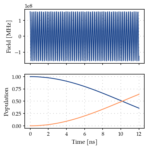
def make_plot():
    """Plot the signal."""
    ts = jnp.linspace(0, t_final, 1001)
    states = jnp.reshape(prop.propagate(ts), (-1, 2))
    sig = cos_envelope(ts, amp=amplitude.get_value()[0], freq=frequency.get_value()[0])

    fig, ax = plt.subplots(2, figsize=(4, 4), sharex=True)
    ax[0].plot(ts / 1e-9, sig)
    ax[0].set_ylabel("Field [MHz]")
    ax[0].grid(True, linestyle=(1, (1, 5)), linewidth=1)

    ax[1].plot(ts / 1e-9, jnp.abs(states) ** 2)
    ax[1].set_ylabel("Population")
    ax[1].grid(True, linestyle=(1, (1, 5)), linewidth=1)

    ax[-1].set_xlabel("Time [ns]")
    return fig, ax


make_plot()

(<Figure size 500x500 with 2 Axes>,
 array([<Axes: ylabel='Field [MHz]'>,
        <Axes: xlabel='Time [ns]', ylabel='Population'>], dtype=object))

3. Gradient based optimisation

While using the above setup one can perform gradient free optimisation. To do a gradient based optimisation, we need to provide the gradient of the Hamiltonian wrt each parameter in the Hamiltonian function.

These gradient functions can be written as analytical functions or constructed using automatic differentiation using jax.grad.

Here we demonstrate both the cases.

1. Analytical functions for gradient of the Hamiltonian.

def grad_amp(t: pq.Array, amp, freq):
    """Gradient of Hamiltonian wrt amplitude."""
    return sigma_x * jnp.cos(freq * t)


def grad_frequency(t: pq.Array, amp, freq):
    """Gradient of Hamiltonian wrt frequency."""
    return -1 * sigma_x * amp * t * jnp.sin(freq * t)


analytical_grad_funcs = [grad_amp, grad_frequency]
tls.gradient_functions = analytical_grad_funcs

2. Gradient functions using Automatic differentiation

from jax import grad

# env_grads(t, amp, freq) returns a tuple of gradients wrt amp and freq
env_grads = grad(cos_envelope, argnums=(1, 2))


def grad_amp(t, amp, freq):
    """Gradient of Hamiltonian wrt amplitude."""
    return sigma_x * env_grads(t, amp, freq)[0]


def grad_freq(t, amp, freq):
    """Gradient of Hamiltonian wrt frequency."""
    return sigma_x * env_grads(t, amp, freq)[1]


tls.gradient_functions = [grad_amp, grad_freq]

zeroone.measure()

0.6404027521371757

4. Create optmap and optimise

from paraqeet.optimisation_map import OptimisationMap
from paraqeet.optimisers.scipy_optimiser_gradient import ScipyOptimiserGradient

optmap = OptimisationMap()
optmap.add(tls)
opt = ScipyOptimiserGradient(zeroone, optimisation_map=optmap)

opt.optimise()

{'status': 1, 'value': 1.4876988529977098e-14, 'iterations': 9, 'message': 'CONVERGENCE: NORM OF PROJECTED GRADIENT <= PGTOL'}

make_plot()

(<Figure size 500x500 with 2 Axes>,
 array([<Axes: ylabel='Field [MHz]'>,
        <Axes: xlabel='Time [ns]', ylabel='Population'>], dtype=object))