DRAG Correction of a Gaussian Pulse

First, we make the necessary imports.

import numpy as np

from paraqeet.optimisation_map import OptimisationMap
from paraqeet.quantity import Quantity
from paraqeet.measurement.unitary_fidelity import UnitaryFidelity
from paraqeet.model.closed_system import ClosedSystem
from paraqeet.model.drive_operator import DriveOperator
from paraqeet.model.transmon import Transmon
from paraqeet.optimisers.scipy_optimiser import ScipyOptimiser
from paraqeet.propagation.scipy_expm_goat import ScipyExpmGOAT
from paraqeet.signal.envelopes import GaussEnvelope
from paraqeet.signal.iq_mixer import IQMixer
from paraqeet.signal.waveform import DRAGMixer

1. Define the Gaussian Tone and put into the DRAGMixer

The GaussTone explicitely allows for the evaluation of an envelope signal and its time derivative which is then used to calculate the DRAG corrected signal in the DRAGMixer

t_final = 20e-9
env_tone = GaussEnvelope()
env_tone.t_final.set_value(t_final)
drag_tone = DRAGMixer(envelopes=env_tone)

gen = IQMixer(envelopes=[drag_tone])

freq = 4.8e9 * 2 * np.pi
anhar = -200e6 * 2 * np.pi

qubit_levels = 3

drive = DriveOperator(gen, is_longitudinal=False)
controlled_transmon = Transmon(
    frequency=Quantity(
        freq,
        min_value=np.array(freq / 4),
        max_value=np.array(freq * 1.2),
        unit="Hz",
        name="Qubit frequency",
    ),
    anharmonicity=Quantity(
        anhar,
        min_value=np.array(anhar * 1.2),
        max_value=np.array(anhar * 0.8),
        unit="Hz",
        name="Qubit anharmonicity",
    ),
    dimension=qubit_levels,
    drives=[drive],
)

model = ClosedSystem(controlled_transmon)

params = gen.get_parameters()

prop = ScipyExpmGOAT(model, res=500e9)
prop.set_initial_state(np.eye(qubit_levels))

params

[Amplitude: 24.7 MHz x 2pi,
 t_final: 20 ns,
 Delta: -1.26 GHz,
 lo_freq: 4.8 GHz x 2pi,
 Phase: 0 rad]

params[0].set_value(3e8)
params[2].set_value(2 * anhar)

gen.get_parameters()

[Amplitude: 47.7 MHz x 2pi,
 t_final: 20 ns,
 Delta: -2.51 GHz,
 lo_freq: 4.8 GHz x 2pi,
 Phase: 0 rad]

2. Set up ideal reference matrix to compare the pulses result to.

def rx(theta) -> np.ndarray:
    """Get the ideal representation of a rx rotation of angle theta."""
    return np.array(
        [
            [np.cos(theta / 2), -1j * np.sin(theta / 2), 0],
            [-1j * np.sin(theta / 2), np.cos(theta / 2), 0],
            [0, 0, 1],
        ],
        dtype=np.complex128,
    )

Set up measure that is optimised. In this case, the gate fidelity between the propagator resulting from the pulse simulation and the ideal reference defined above is used.

gate_fid = UnitaryFidelity(
    propagation=prop,
    gate=rx(np.pi / 2),
    times=np.array([0.0, t_final]),
)

Plot initial pulse shape and population transfer. Target is the full population transfer,i.e., an X-gate.

from plotting import plot_signal_and_dynamics

ts = np.linspace(0.0, t_final, 1001)
plot_signal_and_dynamics(gen, prop, ts, state_labels=[r"$|0\rangle$", r"$|1\rangle$"]);

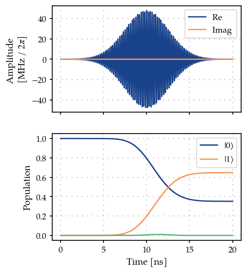
As expected, we get a partial transfer and a low fidelity.

gate_fid.measure()

0.9729714831357765

3. Optimisation

We define an optimizer and link our fidelity measure as a goal function and the parameters of the cosine tone.

optmap = OptimisationMap()
selected_params = []
for i in [0, 2, 3, 4]:
    selected_params.append(params[i])
optmap.add(gen, selected_params)
opt = ScipyOptimiser(gate_fid, optimisation_map=optmap)

opt.optimise()

{'status': 1, 'value': 0.0057610594811500215, 'iterations': 90, 'message': 'CONVERGENCE: RELATIVE REDUCTION OF F <= FACTR*EPSMCH'}

Print all parameters that were optimised.

print("{: >15}: {: >20} {: >20} {: >20}".format("Name", "Value", "Min", "Max"))
print("-" * 80)
for par in selected_params:
    print(
        f"{par.get_name(): >15}: {par.get_value()[0]: >20.6e} "
        f"{par.get_min_value()[0]: >20.6e} {par.get_max_value()[0]: >20.6e}"
    )

           Name:                Value                  Min                  Max
--------------------------------------------------------------------------------
      Amplitude:         2.446330e+08         0.000000e+00         1.000000e+09
          Delta:        -2.495996e+09        -3.769911e+09        -1.256637e+08
        lo_freq:         3.015947e+10         2.412743e+10         3.619115e+10
          Phase:         1.588719e-03        -3.141593e+00         3.141593e+00

Plot final pulse shape and population transfer. Target is the full population transfer,i.e., an X-gate.

plot_signal_and_dynamics(gen, prop, ts, state_labels=[r"$|0\rangle$", r"$|1\rangle$"]);

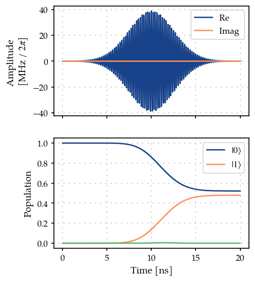
We can see from the plot and optimizer output that we have found better controls. For which the excitement to the second excited state is much smaller than initially.

gate_fid.measure()

0.9942389405232975