Single spin Part 2: Gradient descent gate optimization

First, we make the necessary imports.

import matplotlib.pyplot as plt
import numpy as np

from paraqeet.optimisation_map import OptimisationMap
from paraqeet.quantity import Quantity
from paraqeet.measurement.unitary_fidelity import UnitaryFidelity
from paraqeet.model.closed_system import ClosedSystem
from paraqeet.model.drive_operator import DriveOperator
from paraqeet.model.qubit import Qubit
from paraqeet.optimisers.scipy_optimiser import ScipyOptimiser
from paraqeet.optimisers.scipy_optimiser_gradient import ScipyOptimiserGradient
from paraqeet.propagation.scipy_expm_goat import ScipyExpmGOAT
from paraqeet.signal.envelopes import ConstantEnvelope
from paraqeet.signal.iq_mixer import IQMixer

System Setup

For signal generation, we define a simple cosine shaped tone generator \(A \cos(\omega t)\)

t_final = 10e-9
tone = ConstantEnvelope()
tone.t_final.set_value(t_final)
gen = IQMixer(envelopes=[tone])

We can inspect the pre-defined parameters with

params = gen.get_parameters()

in this case amplitude \(A\) and frequency \(\omega\) and phase \(\phi\).

Next, we setup the qubit system we want to control. We set the qubit frequency \(\omega_q\) to be 4.8 GHz and define the Hamiltonian as

\[H(t)=H_\text{drift}+H_c(t)= \frac{\omega_q}{2} \sigma_z + \Omega(t)\sigma_x\]

, where \(\Omega(t)=A\cos(\omega t+\phi)\) will be supplied by the generator.

freq = 4.327884e9 * 2 * np.pi

drive = DriveOperator(gen, is_longitudinal=False)
controlled_qubit = Qubit(
    frequency=Quantity(
        freq,
        min_value=freq / 4,
        max_value=freq,
        unit="Hz",
        name="Qubit frequency",
    ),
    drives=[drive],
)

model = ClosedSystem(controlled_qubit)

Textbook values for implementing an \(X\) rotation on this system at a time \(T\) would be \(\omega=\omega_q\) and \(A=\pi/T\). We use some offset from these values as initial guess to demonstrate the optimization procedure.

params[0].set_value(0.5 * np.pi / t_final)
params[2].set_value(1.01 * freq)

We select a propagation method, piecewise constant exponentation, and configure \(\sigma_x\) as a target gate. Also we initialize the full basis at time 0 with \(\mathcal{I}_2\)

prop = ScipyExpmGOAT(model, res=500e9)

pauli_x = np.array([[0.0, 1], [1, 0.0]])
pauli_y = np.array([[0.0, -1j], [1j, 0.0]])
pauli_z = np.array([[1, 0], [0.0, -1]])

prop.set_initial_state(np.identity(2))
gate_fid = UnitaryFidelity(
    propagation=prop,
    gate=pauli_x,
    times=np.array([0.0, t_final]),
)

from plotting import plot_signal_and_dynamics

ts = np.linspace(0.0, t_final, 501)
plot_signal_and_dynamics(gen, prop, ts, state_labels=[r"$|0\rangle$", r"$|1\rangle$"]);

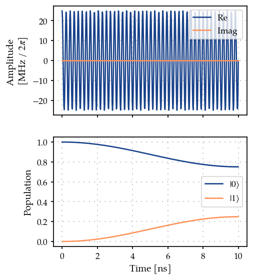
As expected, we get a partial transfer and a low fidelity.

gate_fid.measure()

0.09555411208408474

We define an optimizer and link our fidelity measure as a goal function and the parameters of the cosine tone and optimise just amplitude and frequency, as in the state transfer example.

optmap = OptimisationMap()
optmap.add(gen, [params[0], params[2]])
opt = ScipyOptimiserGradient(gate_fid, optimisation_map=optmap)

opt.optimise()

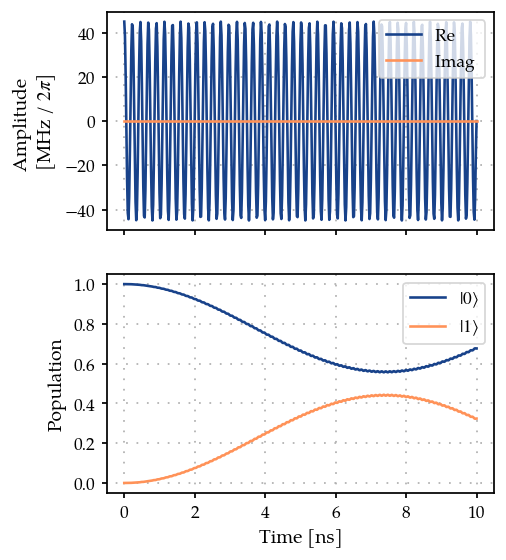
{'status': 1, 'value': 0.8037201693294322, 'iterations': 17, 'message': 'CONVERGENCE: NORM OF PROJECTED GRADIENT <= PGTOL'}

plot_signal_and_dynamics(gen, prop, ts, state_labels=[r"$|0\rangle$", r"$|1\rangle$"]);

Dynamics of Pauli operators

Here, we end up with an unsatisfactory result. For optimising gate fidelities, looking at state populations does not give enough information to identify the problem.

def expecation_value(op, states):
    """Get the expectation value across states."""
    ex = []
    for state in states:
        ex.append(np.real(state.conj() @ op @ state.T))
    return ex

def plot_pauli():
    """Plot the Pauli operators."""
    ts = np.linspace(0, t_final, 1001)
    states = prop.propagate(ts)
    sig = gen.generate_signal(ts) / 1e6 / (2 * np.pi)

    fig, ax = plt.subplots(2, figsize=(4, 4), sharex=True)
    ax[0].plot(ts / 1e-9, sig)
    ax[0].set_ylabel(r"Field [MHz / $2\pi$]")
    ax[0].grid(True, linestyle=(1, (1, 5)), linewidth=1)

    ax[1].plot(ts / 1e-9, expecation_value(pauli_x, states[:, :, 0]))
    ax[1].plot(ts / 1e-9, expecation_value(pauli_y, states[:, :, 0]))
    ax[1].plot(ts / 1e-9, expecation_value(pauli_z, states[:, :, 0]))
    ax[1].set_ylabel(r"Expectation value $\langle\hat\sigma_i\rangle$")
    ax[1].grid(True, linestyle=(1, (1, 5)), linewidth=1)

    ax[-1].set_xlabel("Time [ns]")
    ax[1].legend(["X", "Y", "Z"])
    return fig, ax


plot_pauli()

(<Figure size 500x500 with 2 Axes>,
 array([<Axes: ylabel='Field [MHz / $2\pi$]'>,
        <Axes: xlabel='Time [ns]', ylabel='Expectation value $\langle\hat\sigma_i\rangle$'>],
       dtype=object))

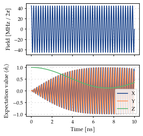
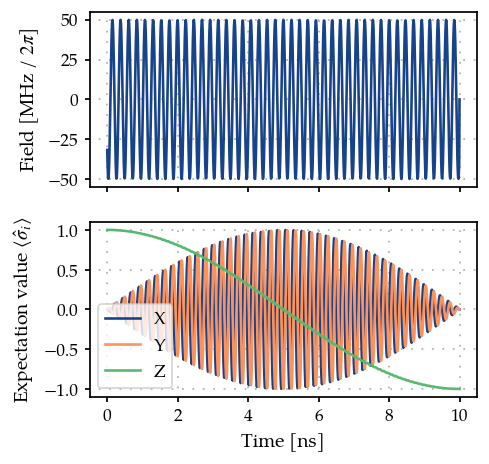
Instead, we look at the expecation values of the three Pauli operators and observe that the qubit is rotating at its eigenfrequency along the Z-axis. We can mitigate this problem by allowing the rotation axis of our drive to shift and inclide the phase parameter in the optimisation.

optmap = OptimisationMap()
optmap.add(tone, [params[0], params[2], params[3]])
opt = ScipyOptimiser(gate_fid, optimisation_map=optmap)

params[0].set_value(0.5 * np.pi / t_final)
params[2].set_value(1.01 * freq)
opt.optimise()

{'status': 1, 'value': 1.0475176281943277e-11, 'iterations': 108, 'message': 'CONVERGENCE: RELATIVE REDUCTION OF F <= FACTR*EPSMCH'}

plot_pauli()

(<Figure size 500x500 with 2 Axes>,
 array([<Axes: ylabel='Field [MHz / $2\pi$]'>,
        <Axes: xlabel='Time [ns]', ylabel='Expectation value $\langle\hat\sigma_i\rangle$'>],
       dtype=object))