Arbitrary bosonic state preparation using GRAPE
In this notebook, we implement a standard application of GRAPE, namely the preparation of an arbitrary state of a bosonic mode, such a resonant mode of a microwave cavity. In the notebook, we mostly follow the optimization strategy of [Heeres2017]. The parameters are taken from [Eickbusch2022] Table S1, without considering the anharmonicity for simplicity and with the exception of the dispersive shift taken to be \(10\) times larger for simulation purposes. Our starting point is the well-known Jaynes-Cummings Hamiltonian in the dispersive regime, which describes an interaction of a qubit with a single bosonic mode when the characteristic qubit frequency \(\omega_{q}\) is far detuned from the one of the resonator \(\omega_{r}\) (see for instance [Blais2021] for more details)
where we set \(\hbar = 1\). The parameter \(\chi\) is the dispersive shift, which represents a qubit-state-dependent shift of the frequency of the resonator. Note that we set conventionally \(\sigma_z = | e \rangle \langle e | - |g \rangle \langle g |\), with \(|e \rangle, |g \rangle\) the excited and ground state of the qubit, respectively. We additionally introduce a drive Hamiltonian on both the qubit and the resonator mode, which we write directly within the rotating wave approximation
The total Hamiltonian is
We assume that the qubit and the resonator are both driven resonantly, i.e., \(\omega_{d, q} = \omega_q\) and \(\omega_{d,r}=\omega_r\), and work in the interaction picture (rotating frame) with reference Hamiltonian
so that the Hamiltonian in the interaction picture is
Our goal is to prepare the resonator in a Fock state \(| n \rangle, \, n \in \mathbb{N}\), while keeping the qubit in the ground state \(| g \rangle\). Thus, the target state is
In the notebook, \(n\) is set to \(2\) as an example. We assume that the system starts in the initial state
Let \(\varepsilon(t) = (\varepsilon_{r}(t), \varepsilon_{q}(t))\). For a fixed time \(T\), the system evolves to a state \(| \Psi(T; \varepsilon(t)) \rangle = U(T; \varepsilon(t)) | \Psi_{\mathrm{initial}} \rangle\). We thus want to maximize the state fidelity, i.e., the overlap between \(| \Psi_{\mathrm{target}} \rangle\) and \(| \Psi(t) \rangle\):
In GRAPE we consider piecewise constant pulses with time step \(\Delta t\). Each constant can take values in a certain subset \(\mathcal{I} \in \mathbb{C}\). We denote by \(R\) the range of the piecewise constant pulse, i.e., \(R = \mathrm{max}_{\varepsilon, \varepsilon' \in \mathcal{I}} | \varepsilon - \varepsilon'|\). Thus, in what follows \(R_r\) and \(R_q\) represent the range of the resonator and qubit pulses, respectively.
import numpy as np
import matplotlib.pyplot as plt

from paraqeet.quantity import Quantity
from paraqeet.model.resonator import Resonator
from paraqeet.model.qubit import Qubit
from paraqeet.model.coupling import Coupling
from paraqeet.signal.envelopes import GaussEnvelope
from paraqeet.signal.pwc_generator import PWCGenerator
from paraqeet.model.closed_system import ClosedSystem
from paraqeet.model.rotating_frame_drive import RotatingFrameDrive
from paraqeet.model.composite_hamiltonian import CompositeHamiltonian
from paraqeet.measurement.state_transfer_fidelity import StateTransferFidelityGRAPE
from paraqeet.measurement.weighted_sum_goal import WeightedSumGoal
from paraqeet.propagation.scipy_expm_grape import ScipyExpmGRAPE
from paraqeet.optimisation_map import OptimisationMap
from paraqeet.optimisers.scipy_optimiser_gradient import ScipyOptimiserGradient
from paraqeet.measurement.smoothness import Smoothness
We initialize our pulses as simple Gaussian envelopes. Additionally, we require fix ranges for the minimum and maximum amplitudes.
# in seconds (See Eickbusch et al https://arxiv.org/abs/2111.06414 S9 A)
delta_sampling = 33e-9
n_pwc = 40  # number of piecewiise constants in the pulse
t_final = n_pwc * delta_sampling  # for now just set up for trying
tlist = np.linspace(0, t_final, n_pwc + 1)
eps_res = 2 * np.pi * 1.0  # initial amplitude of the resonator (in MHz)
eps_max_res = 5 * eps_res  # maximum amplitude of the resonator (in MHz)
eps_qubit = 2 * np.pi * 1.0  # initial amplitude of the qubit (in MHz)
eps_max_qubit = 5 * eps_qubit  # maximum amplitude of the resonator (in MHz)
tone_res = GaussEnvelope(
    amplitude=Quantity(eps_res * 1e6, -eps_max_res * 1e6, eps_max_res * 1e6),
    t_final=Quantity(t_final, 1 / 2 * t_final, 2 * t_final),
)
tone_qubit = GaussEnvelope(
    amplitude=Quantity(eps_qubit * 1e6, -eps_max_qubit * 1e6, eps_max_qubit * 1e6),
    t_final=Quantity(t_final, 1 / 2 * t_final, 2 * t_final),
)
gen_res = PWCGenerator(envelopes=[tone_res], tlist=tlist)
gen_res.multiply_flat_top = True

gen_qubit = PWCGenerator(envelopes=[tone_qubit], tlist=tlist)
gen_qubit.multiply_flat_top = True
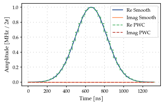
We plot the resonator tone and compare it to its smooth version. Similarly one can plot the qubit tone.
from plotting import plot_signal

ts = np.linspace(0, t_final, 1001)
fig, ax = plt.subplots(1, figsize=(5, 3))

plot_signal(tone_res, ts, ax, linestyle="-", label="Smooth")
plot_signal(gen_res, ts, ax, linestyle="--", label="PWC")

plt.legend()
plt.show()
We define qubit and resonator parameters, as well as the list of different Fock truncation numbers. We also set the target Fock state.
For now we set the Fock-state truncation at small values (3 and 4) for testing the method. Later we demonstrate the method with (30 and 31) levels in the resonator.
# Increasing the number of Fock states gives a more realistic scenario, at the price of increasing the simulation time
n_fock_truncation_list = [3, 4]
fock_target = 2
n_times = 1001

omega_range_factor = 1e-3  # just for initialization of the Quantity object
omega_res = 2 * np.pi * 5.26e9
omega_qubit = 2 * np.pi * 6.65e9

omega_drive_res = omega_res
omega_drive_qubit = omega_qubit

detuning_drive_res = omega_res - omega_drive_res
detuning_drive_qubit = omega_qubit - omega_drive_qubit

drive_res = RotatingFrameDrive(gen_res)
drive_qubit = RotatingFrameDrive(gen_qubit)
Due to the infinite-dimensional nature of the Hilbert space of the resonator, it is necessary to introduce a Fock state truncation number \(N_{\mathrm{T}}\). This creates the problem that given certain pulses \(\mathcal{F}\) depends on the choice of \(N_{\mathrm{T}}\). Following [Heeres2017], we thus consider \(N_{\mathrm{T}} \in \{N_{\mathrm{T}}^{(\mathrm{min})}, N_{\mathrm{T}}^{(\mathrm{min})} + 1, \dots, N_{\mathrm{T}}^{(\mathrm{max})} \}\), and introduce a penalty when having different values of fidelities for different truncation numbers. Thus, we create different systems, and accordingly fidelity measures, for the different Fock truncation numbers.
def create_experiment(n_fock_truncation_list, fock_target):
    """
    Create the inital and target states, for the given Fock numbers.
    Also create the propagations and measurements for the given truncation numbers and target Fock states.
    """
    resonator_list = []
    coupling_list = []
    model_list = []
    hamiltonian_list = []
    prop_list = []
    initial_state_list = []
    target_state_list = []
    fock_number_op_list = []
    fid_list = []

    qubit = Qubit(
        frequency=Quantity(
            value=detuning_drive_qubit,
            min_value=-omega_range_factor * omega_qubit,
            max_value=omega_range_factor * omega_qubit,
        ),
        drives=[drive_qubit],
    )
    ground_state_qubit = np.array([[0.0], [1.0]])

    # We take it to be 10 times the value in Eickbusch et al to speed up the simulation
    chi = 2 * np.pi * 32.81e3 * 10

    for n in n_fock_truncation_list:
        resonator = Resonator(
            frequency=Quantity(
                value=detuning_drive_res,
                min_value=-omega_range_factor * omega_res,
                max_value=omega_range_factor * omega_res,
            ),
            dimension=n,
            drives=[drive_res],
        )
        resonator_list.append(resonator)
        coupling = Coupling(
            [resonator, qubit],
            is_longitudinal=True,
            coefficient=Quantity(value=chi, min_value=chi / 2, max_value=2 * chi),
        )
        coupling_list.append(coupling)
        ham = CompositeHamiltonian([resonator, qubit], [coupling])
        hamiltonian_list.append(ham)
        model = ClosedSystem(hamiltonian=ham)
        model_list.append(model)
        prop = ScipyExpmGRAPE(model, res=1e9)

        initial_res_state = np.zeros([n, 1], dtype=complex)
        initial_res_state[0, 0] = 1  # vacuum state
        initial_state = np.kron(initial_res_state, ground_state_qubit)
        initial_state_list.append(initial_state)

        target_res_state = np.zeros([n, 1], dtype=complex)
        target_res_state[fock_target, 0] = 1
        target_state = np.kron(target_res_state, ground_state_qubit)
        target_state_list.append(target_state)

        n_op = np.kron(np.diag([x for x in range(n)]), np.identity(2))
        fock_number_op_list.append(n_op)

        prop.set_initial_state(initial_state)
        prop.target_state = target_state
        prop.use_schirmer_derivative = True

        prop_list.append(prop)

        fid = StateTransferFidelityGRAPE(
            propagation=prop, initial_state=initial_state, target_state=target_state, times=tlist
        )

        fid_list.append(fid)

    return initial_state_list, target_state_list, fock_number_op_list, prop_list, fid_list


initial_state_list, target_state_list, fock_number_op_list, prop_list, meas_list = create_experiment(
    n_fock_truncation_list, fock_target
)
Furthermore, following [Heeres2017] we also introduce a penalty for non-smooth pulses. In particular, we consider the (normalized) sum of consecutive square differences of the pulse pixels as cost function (see Eqs. 21 in the supplementary material of [Heeres2017]) for both the resonator and the qubit pulses:
res_smoothness = Smoothness(pwc_generator=gen_res)
qubit_smoothness = Smoothness(pwc_generator=gen_qubit)
meas_list.append(res_smoothness)
meas_list.append(qubit_smoothness)
We consider as cost function of the form
that we want to maximize. This cost weighted cost function can be constructed using the class WeightedSumGoal.
weights = np.array([1.0 for _ in range(len(meas_list))])
weights[-1] = 10.0
weights[-2] = 10.0
weight_sum_of_squares = -0.05
total_sum_of_weights = np.sum(weights) + weight_sum_of_squares
weights = weights / total_sum_of_weights
weight_sum_of_squares = weight_sum_of_squares / total_sum_of_weights
meas_list_bool = [True for meas in meas_list]
meas_list_bool[-1] = False
meas_list_bool[-2] = False
sum_of_squares_options = {"weight": weight_sum_of_squares, "meas_bool": meas_list_bool}

goal = WeightedSumGoal(meas_list, weights, sum_of_squares_options=sum_of_squares_options)
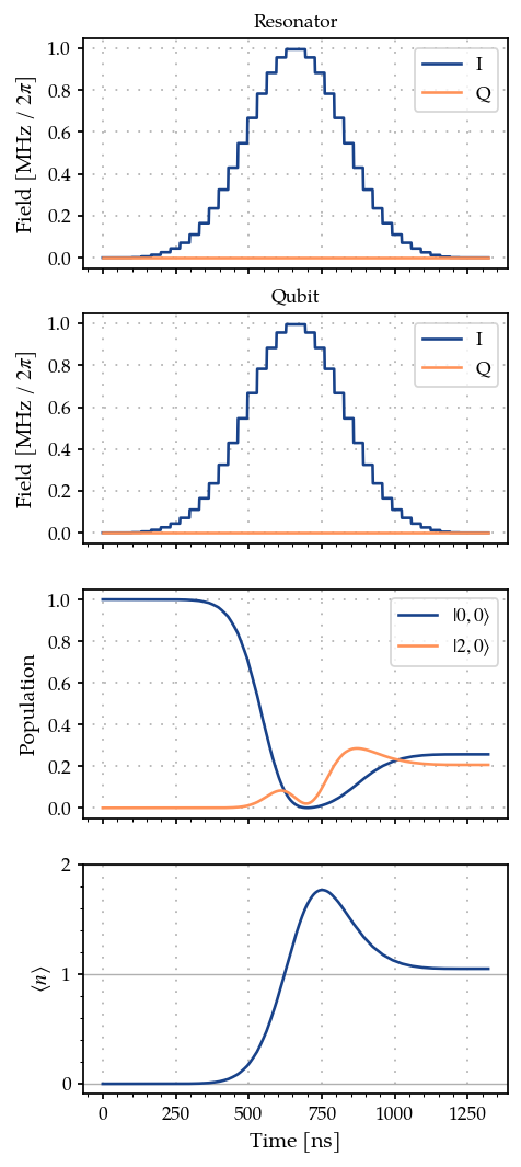
We can plot the initial pulses, as well as the corresponding relevant dynamics.
def plot_states_and_fock_number(item=0):
    """Plot the states."""
    ts = np.linspace(0, t_final, n_times)
    states = prop_list[item].propagate(ts)
    sig_res = gen_res.generate_signal(ts)
    sig_qubit = gen_qubit.generate_signal(ts)
    pop_initial_state = (np.abs(initial_state_list[item].conj().T @ states) ** 2).flatten()
    pop_target_state = (np.abs(target_state_list[item].conj().T @ states) ** 2).flatten()

    pop_initial_state = (np.abs(initial_state_list[item].conj().T @ states) ** 2).flatten()

    n_fock_avg = np.zeros(n_times, dtype=float)
    for k in range(n_times):
        n_fock_avg[k] = np.real((states[k].conj().T @ fock_number_op_list[item] @ states[k])[0, 0])

    _, ax = plt.subplots(4, figsize=(4, 10), sharex=True)
    ax[0].plot(ts / 1e-9, np.real(sig_res) / 1e6 / (2 * np.pi), label="I")
    ax[0].plot(ts / 1e-9, np.imag(sig_res) / 1e6 / (2 * np.pi), label="Q")
    ax[0].legend(loc=1)
    ax[0].set_ylabel(r"Field [MHz / $2\pi$]")
    ax[0].set_title("Resonator")
    ax[0].grid(True, linestyle=(1, (1, 5)), linewidth=1)

    ax[1].plot(ts / 1e-9, np.real(sig_qubit) / 1e6 / (2 * np.pi), label="I")
    ax[1].plot(ts / 1e-9, np.imag(sig_qubit) / 1e6 / (2 * np.pi), label="Q")
    ax[1].legend(loc=1)
    ax[1].set_ylabel(r"Field [MHz / $2\pi$]")
    ax[1].set_title("Qubit")
    ax[1].grid(True, linestyle=(1, (1, 5)), linewidth=1)

    ax[2].plot(ts / 1e-9, pop_initial_state, label="$|0,0 \\rangle$")
    ax[2].plot(ts / 1e-9, pop_target_state, label="$|2, 0 \\rangle$")
    ax[2].legend(loc="best")
    ax[2].set_ylabel("Population")
    ax[2].grid(True, linestyle=(1, (1, 5)), linewidth=1)

    ax[3].plot(ts / 1e-9, n_fock_avg)
    ax[3].set_ylabel("$\\langle n \\rangle$")
    if n_fock_truncation_list[item] < 10:
        y_fock_ticks = np.arange(n_fock_truncation_list[item])
    else:
        y_fock_ticks = np.arange(n_fock_truncation_list[item])[::5]
    ax[3].set_yticks(y_fock_ticks)
    ax[3].grid(axis="y", which="major")
    ax[3].minorticks_on()
    ax[3].grid(True, axis="x", linestyle=(1, (1, 5)), linewidth=1)

    ax[-1].set_xlabel("Time [ns]")
    plt.show()


plot_states_and_fock_number()
We can compute the fidelities for the different truncation numbers
print(f"Fidelity at N_T={n_fock_truncation_list[0]} = {meas_list[0].measure()}")
print(f"Fidelity at N_T={n_fock_truncation_list[1]} = {meas_list[1].measure()}")
Fidelity at N_T=3 = 0.2067436053211263
Fidelity at N_T=4 = 0.14197098648890233
which are quite poor! We now proceed with the pulse optimization.
max_iter = 1000  # set to 1000 for a good result; set to 10 for a quick example
optmap = OptimisationMap()
optmap.add(gen_res, gen_res.get_parameters())
optmap.add(gen_qubit, gen_qubit.get_parameters())
opt = ScipyOptimiserGradient(goal, optimisation_map=optmap)
opt.set_options({"maxfun": max_iter})
optmap.register_params_with_optimisables()
optmap
==== <class 'paraqeet.signal.pwc_generator.PWCGenerator'> ====
[Inphase: [3.13e+03, 6.69e+03, 1.37e+04, 2.71e+04, 5.15e+04, 9.38e+04, 1.64e+05, 2.76e+05, 4.46e+05, 6.93e+05, 1.03e+06, 1.48e+06, 2.04e+06, 2.7e+06, 3.43e+06, 4.19e+06, 4.92e+06, 5.54e+06, 6.01e+06, 6.25e+06, 6.25e+06, 6.01e+06, 5.54e+06, 4.92e+06, 4.19e+06, 3.43e+06, 2.7e+06, 2.04e+06, 1.48e+06, 1.03e+06, 6.93e+05, 4.46e+05, 2.76e+05, 1.64e+05, 9.38e+04, 5.15e+04, 2.71e+04, 1.37e+04, 6.69e+03, 3.13e+03], out-of-phase: [0, 0, 0, 0, 0, 0, 0, 0, 0, 0, 0, 0, 0, 0, 0, 0, 0, 0, 0, 0, 0, 0, 0, 0, 0, 0, 0, 0, 0, 0, 0, 0, 0, 0, 0, 0, 0, 0, 0, 0]]
%%time
opt.optimise()
CPU times: user 2min 25s, sys: 1.41 s, total: 2min 27s
Wall time: 41.7 s
{'status': 1, 'value': 0.004241814930537657, 'iterations': 158, 'message': 'CONVERGENCE: RELATIVE REDUCTION OF F <= FACTR*EPSMCH'}
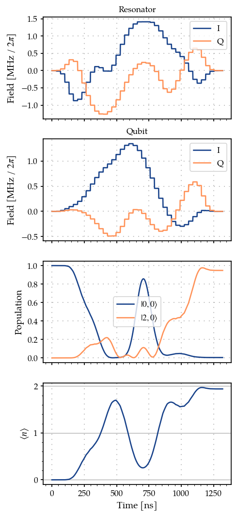
We can now plot the new pulses and the corresponding dynamics. If the number of iterations (max_iter) is chosen to be large enough, we should see an improvement.
plot_states_and_fock_number()
The new fidelities are
print(f"Fidelity at N_T={n_fock_truncation_list[0]} = {meas_list[0].measure()}")
print(f"Fidelity at N_T={n_fock_truncation_list[1]} = {meas_list[1].measure()}")
Fidelity at N_T=3 = 0.9475693477178125
Fidelity at N_T=4 = 0.9631119242149566
Setting truncation to higher values
Here we increase the system truncation to 30 and 31 levels and rerun the entire simulation.
Note - The following takes about 10-15 mins to run on an AMD-EPYC Milan processor with 128 cores and 256GB RAM (might take more depending on the number of CPU cores available).
We first reset the generator parameters (by redefining them), and redefine the resonator with higher truncation numbers.
# in seconds (See Eickbusch et al https://arxiv.org/abs/2111.06414 S9 A)
delta_sampling = 33e-9
n_pwc = 40  # number of piecewiise constants in the pulse
t_final = n_pwc * delta_sampling  # for now just set up for trying
tlist = np.linspace(0, t_final, n_pwc + 1)
eps_res = 2 * np.pi * 1.0  # initial amplitude of the resonator (in MHz)
eps_max_res = 5 * eps_res  # maximum amplitude of the resonator (in MHz)
eps_qubit = 2 * np.pi * 1.0  # initial amplitude of the qubit (in MHz)
eps_max_qubit = 5 * eps_qubit  # maximum amplitude of the resonator (in MHz)
tone_res = GaussEnvelope(
    amplitude=Quantity(eps_res * 1e6, -eps_max_res * 1e6, eps_max_res * 1e6),
    t_final=Quantity(t_final, 1 / 2 * t_final, 2 * t_final),
)
tone_qubit = GaussEnvelope(
    amplitude=Quantity(eps_qubit * 1e6, -eps_max_qubit * 1e6, eps_max_qubit * 1e6),
    t_final=Quantity(t_final, 1 / 2 * t_final, 2 * t_final),
)
gen_res = PWCGenerator(envelopes=[tone_res], tlist=tlist)
gen_qubit = PWCGenerator(envelopes=[tone_qubit], tlist=tlist)
n_fock_truncation_list = [30, 31]
fock_target = 2
n_times = 1001

omega_range_factor = 1e-3  # just for initialization of the Quantity object
omega_res = 2 * np.pi * 5.26e9
omega_qubit = 2 * np.pi * 6.65e9

omega_drive_res = omega_res
omega_drive_qubit = omega_qubit

detuning_drive_res = omega_res - omega_drive_res
detuning_drive_qubit = omega_qubit - omega_drive_qubit

drive_res = RotatingFrameDrive(gen_res)
drive_qubit = RotatingFrameDrive(gen_qubit)

initial_state_list, target_state_list, fock_number_op_list, prop_list, meas_list = create_experiment(
    n_fock_truncation_list, fock_target
)
lets also add the smoothness penalty to the measurement
res_smoothness = Smoothness(pwc_generator=gen_res)
qubit_smoothness = Smoothness(pwc_generator=gen_qubit)
meas_list.append(res_smoothness)
meas_list.append(qubit_smoothness)

weights = np.array([1.0 for _ in range(len(meas_list))])
weights[-1] = 10.0
weights[-2] = 10.0
weight_sum_of_squares = -0.05
total_sum_of_weights = np.sum(weights) + weight_sum_of_squares
weights = weights / total_sum_of_weights
weight_sum_of_squares = weight_sum_of_squares / total_sum_of_weights
meas_list_bool = [True for meas in meas_list]
meas_list_bool[-1] = False
meas_list_bool[-2] = False
sum_of_squares_options = {"weight": weight_sum_of_squares, "meas_bool": meas_list_bool}

goal = WeightedSumGoal(meas_list, weights, sum_of_squares_options=sum_of_squares_options)
And then plot the dynamics of the resonator under the unoptimised pulse
plot_states_and_fock_number()
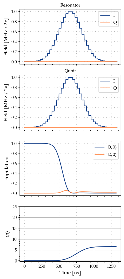
Initial fidelity before optimisation
print(f"Fidelity at N_T={n_fock_truncation_list[0]} = {meas_list[0].measure()}")
print(f"Fidelity at N_T={n_fock_truncation_list[1]} = {meas_list[1].measure()}")
Fidelity at N_T=30 = 0.0191897809908802
Fidelity at N_T=31 = 0.019189780990880208
We redefine the optimiser and perform the optimisation again with higher truncation numbers
max_iter = 1000  # set to 1000 for a good result; set to 10 for a quick example
optmap = OptimisationMap()
optmap.add(gen_res, gen_res.get_parameters())
optmap.add(gen_qubit, gen_qubit.get_parameters())
opt = ScipyOptimiserGradient(goal, optimisation_map=optmap)
opt.set_options({"maxfun": max_iter})
optmap.register_params_with_optimisables()
%%time
opt.optimise()
CPU times: user 8h 23min 39s, sys: 23min 41s, total: 8h 47min 21s
Wall time: 11min 46s
{'status': 1, 'value': 0.003695502233559078, 'iterations': 269, 'message': 'CONVERGENCE: RELATIVE REDUCTION OF F <= FACTR*EPSMCH'}
The new fidelities are
print(f"Fidelity at N_T={n_fock_truncation_list[0]} = {meas_list[0].measure()}")
print(f"Fidelity at N_T={n_fock_truncation_list[1]} = {meas_list[1].measure()}")
Fidelity at N_T=30 = 0.9756092572351025
Fidelity at N_T=31 = 0.9755700654718467
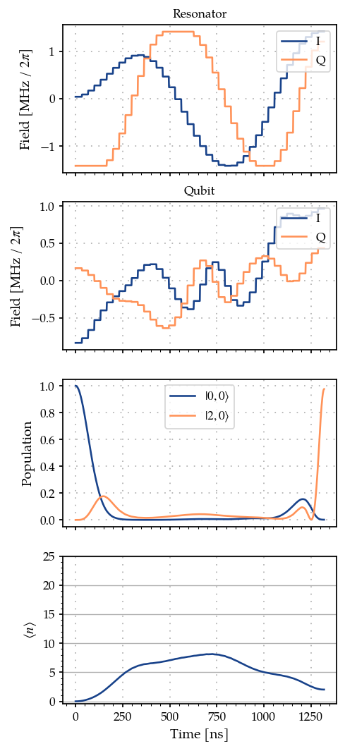
And the dynamics of the system under these optimised pulses looks like the following
plot_states_and_fock_number()