Single spin Part 3: Single qubit gate optimization using GRAPE

1. Generate a PWC pulse shape

import matplotlib.pyplot as plt
import numpy as np

from paraqeet.quantity import Quantity
from paraqeet.signal.envelopes import GaussEnvelope
from paraqeet.signal.pwc_generator import PWCGenerator

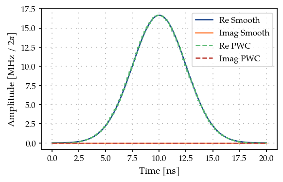
First, let’s generate a piecewise constant (PWC) pulse envelope for the Gaussian pulse

t_final = 20e-9
tlist = np.linspace(0, t_final, 101)
tone = GaussEnvelope(amplitude=Quantity(2 * np.pi / t_final / 3, -5 * np.pi / t_final, 5 * np.pi / t_final))
tone.t_final.set_value(t_final)
gen = PWCGenerator(envelopes=[tone], tlist=tlist)
gen.multiply_flat_top = True

params = gen.get_parameters()

from plotting import plot_signal

ts = np.linspace(0, t_final, 501)
fig, ax = plt.subplots(1, figsize=(5, 3))
plot_signal(tone, ts, ax, linestyle="-", label="Smooth")
plot_signal(gen, ts, ax, linestyle="--", label="PWC")
ax.legend(loc=1, frameon=True)
plt.show()

2. Define Hamiltonian in the rotating frame of drive

Next, we setup the qubit system we want to control. We define the Hamiltonian in the rotating frame of drive such that the pulse oscillates slowly to apply GRAPE gradients.

The Hamiltonain in the rotating frame of the drive is given by -

\[H(t) = \big(\omega_q - \omega_d\big) b^\dagger b -\frac{\alpha}{2} (b^\dagger)^2 b^2 + (\epsilon(t) b + \epsilon(t)^* b)\]

from paraqeet.model.closed_system import ClosedSystem
from paraqeet.model.rotating_frame_drive import RotatingFrameDrive
from paraqeet.model.transmon import Transmon
from paraqeet.quantity import Quantity

freq = 7.86e9 * 2 * np.pi
dims = 3
anharm = -50e6 * 2 * np.pi
offset = 5e6 * 2 * np.pi

drive_freq = freq + offset
qubit_freq = freq - drive_freq

Drive = RotatingFrameDrive(gen)
transmon = Transmon(
    frequency=Quantity(
        qubit_freq,
        1.2 * qubit_freq,
        0.8 * qubit_freq,
        unit="Hz",
        name="Frequency",
    ),
    anharmonicity=Quantity(anharm, 1.2 * anharm, 0.8 * anharm, unit="Hz", name="Anharmonicity"),
    drives=[Drive],
    dimension=dims,
)

model = ClosedSystem(transmon)

from paraqeet.measurement.state_transfer_fidelity import StateTransferFidelityGRAPE
from paraqeet.propagation.scipy_expm_grape import ScipyExpmGRAPE

prop = ScipyExpmGRAPE(model, resolution=1e9)

init = np.array([[1.0], [0.0], [0.0]])  # |0>
target = np.array([[0.0], [1.0], [0.0]])  # |1>

times = np.array([0.0, t_final])

prop.set_initial_state(init)
prop.set_target_state(target)

prop.use_schirmer_derivative = True

zeroone = StateTransferFidelityGRAPE(
    propagation=prop,
    initial_state=init,
    target_state=target,
)

from plotting import plot_signal_and_dynamics

ts = np.linspace(0.0, t_final, 101)
plot_signal_and_dynamics(gen, prop, ts, state_labels=[r"$|0\rangle$", r"$|1\rangle$"]);

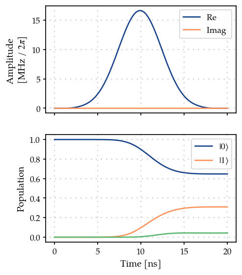
As expected, we get a partial transfer and a low fidelity.

zeroone.measure(times)

0.7449176579124753

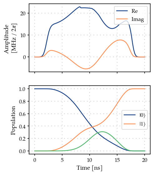
3. Opimisation

We define an optimizer and link our fidelity measure as a goal function and the parameters of the cosine tone and optimize just amplitude and frequency, as in the state transfer example.

from paraqeet.optimization_map import OptimizationMap
from paraqeet.optimizers.scipy_optimizer_gradient import ScipyOptimizerGradient

optmap = OptimizationMap()
optmap.add(gen, params)
opt = ScipyOptimizerGradient(zeroone, optimization_map=optmap)

opt.optimize(gen.tlist)

{'status': 1, 'value': 4.911978601640499e-09, 'iterations': 14, 'message': 'CONVERGENCE: NORM OF PROJECTED GRADIENT <= PGTOL'}

plot_signal_and_dynamics(gen, prop, ts, state_labels=[r"$|0\rangle$", r"$|1\rangle$"]);