Optimal control of a single spin by using GOAT over GRAPE

In this introductory example we compute the gradients of analytic pulse shapes in GOAT by using the gradients of the time evolution from GRAPE. This is performed by using chain rule -

\[\frac{\partial J}{\partial p} = \sum_k \frac{\partial J}{\partial c_k} \frac{\partial c_k}{\partial p}\]

where \(c_k = c(t_k)\) the ‘pixelated’ control pulse, \(\vec{p}\) are the analytical parameters of the control pulse \(c(t) \equiv c(\vec{p}, t)\), and \(\frac{\partial J}{\partial c_k}\) are the gradients from GRAPE.

1. Generate a PWC pulse shape

import jax.numpy as jnp
import matplotlib.pyplot as plt
import numpy as np

from paraqeet.quantity import Quantity
from paraqeet.signal.envelopes import FlatTopGaussianEnvelope
from paraqeet.signal.pwc_generator import PWCGenerator
from paraqeet.signal.waveform import FlatTopGaussianFilter

Define the FlatTopGaussianEnvelope and the PWCGenerator. The PWCGenerator is used to produce the pixelated pulse shape for computing the gradients using GRAPE.

Here we also define the FlatTopGaussianFilter to ensure that the pulse always starts and end at zero.

The optimization would be performed on the FlatTopGaussianEnvelope parameters: amplitude, t_up, t_down, ramp_time.

t_final = 20e-9
num_pwc = 30  # number of signal pixels
t_simu = t_final
times = np.linspace(0, t_final, num_pwc)

tone = FlatTopGaussianEnvelope(
    amplitude=Quantity(np.pi / t_final / 3, -np.pi / t_final, np.pi / t_final, name="Amplitude"),
    t_up=Quantity(1e-9, 0.0, t_final, name="t_up"),
    t_down=Quantity(t_final - 1e-9, 0.0, t_final, name="t_down"),
    ramp_time=Quantity(1e-9, 0.5e-9, t_final, name="ramp_time"),
)

filtered_tone = FlatTopGaussianFilter(tone, t_final=Quantity(t_final, 0.0, 1.2 * t_final, name="t_final"))

gen = PWCGenerator(envelopes=[filtered_tone], tlist=times)

params = gen.get_parameters()
params[0].set_limits(-200e6, 200e6)
params[1].set_limits(-200e6, 200e6)

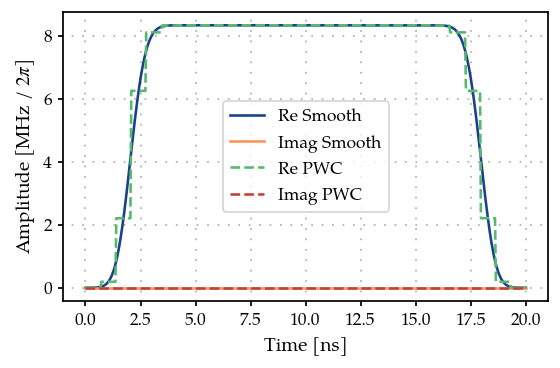
from plotting import plot_signal

ts = np.linspace(0, t_final, 501)
fig, ax = plt.subplots(1, figsize=(5, 3))

plot_signal(filtered_tone, ts, ax, linestyle="-", label="Smooth")
plot_signal(gen, ts, ax, linestyle="--", label="PWC");

2. Define Hamiltonian in the rotating frame of drive

As a simple toy model, we use a single spin.

from paraqeet.model.closed_system import ClosedSystem
from paraqeet.model.differentiable_hamiltonian import DifferentiableHamiltonian
from paraqeet.model.rotating_frame_drive import RotatingFrameDrive
from paraqeet.quantity import Array


class SpinRWA(DifferentiableHamiltonian):
    """A Single Spin."""

    def __init__(self, drives=None):
        super().__init__(drives)
        self.sigma_p = jnp.array([[0j, 1], [0, 0]])
        self.dim = 2

    def get_value_at_timestep(self, timestep: float) -> Array:
        """Just sigma-X."""
        return self._drives[0].get_value_at_timestep(self.sigma_p, timestep)

    def get_value_and_gradient(self, times: Array) -> tuple[Array, Array] | tuple[float, Array]:
        """Gradient is just the drive matrix."""
        return self.get_value(times), self._drives[0].get_gradient(self.sigma_p, times)

    def get_gradient_at_timestep(self, time):
        """Computes the gradient"""
        return self._drives[0].get_gradient_at_timestep(self.sigma_p, time)

    def dimension(self) -> int:
        """Returns the dimension"""
        raise self.d

    def get_collapseops(self) -> list[tuple[Array, Array]]:
        """Returns an empyt list since we study closed system dynamics"""
        return []

    def get_parameters(self):
        """Returns the parameters, which in this case are only the drive parameters"""
        return self._get_drive_parameters()


drive = RotatingFrameDrive(gen)
spin = SpinRWA(drives=[drive])
model = ClosedSystem(spin)

Using GRAPE as the method to propagate and compute the gradients

from paraqeet.measurement.state_transfer_fidelity import StateTransferFidelityGRAPE
from paraqeet.propagation.scipy_expm_grape import ScipyExpmGRAPE

prop = ScipyExpmGRAPE(model, resolution=2e9)

init = np.array([[1.0], [0.0]])  # |0>
target = np.array([[0.0], [1.0]])  # |1>

prop.set_initial_state(init)
prop.set_target_state(target)

zeroone = StateTransferFidelityGRAPE(
    propagation=prop,
    initial_state=init,
    target_state=target,
)

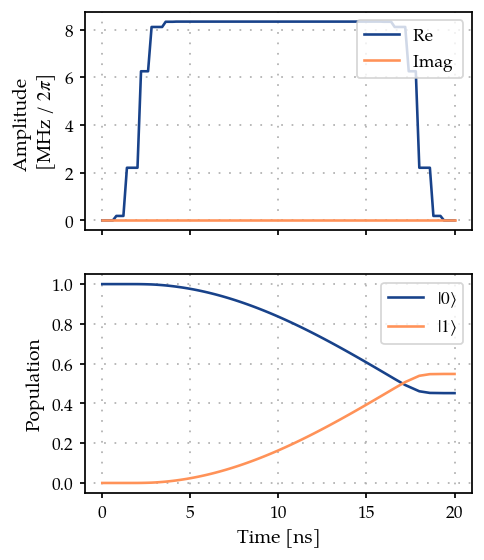
zeroone.measure(times)

0.5458431639927377

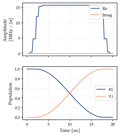
from plotting import plot_signal_and_dynamics

ts = np.linspace(0.0, t_final, 101)
plot_signal_and_dynamics(gen, prop, ts, state_labels=[r"$|0\rangle$", r"$|1\rangle$"]);

3. Optimization

Finally, we define the GOATOverGRAPE fideltiy that chains together the GRAPE gradients to compute the gradient wrt the tone parameters

from paraqeet.measurement.goat_over_grape import GOATOverGRAPE
from paraqeet.optimization_map import OptimizationMap
from paraqeet.optimizers.scipy_optimizer_gradient import ScipyOptimizerGradient

optmap = OptimizationMap()
optmap.add(filtered_tone)
optmap.register_params_with_optimizables()

goat = GOATOverGRAPE(zeroone, prop, gen)
opt_grad = ScipyOptimizerGradient(goat, optimization_map=optmap)

opt_grad.optimize(np.array([0.0, t_simu]))

{'status': 1, 'value': 3.1086244689504383e-15, 'iterations': 6, 'message': 'CONVERGENCE: NORM OF PROJECTED GRADIENT <= PGTOL'}

For this simple example, we reach near perfect fidelity within a few iterations.

plot_signal_and_dynamics(gen, prop, ts, state_labels=[r"$|0\rangle$", r"$|1\rangle$"]);