Gradient-based optimization of a cross-resonance gate between two transmons

import itertools

import matplotlib.pyplot as plt
import numpy as np

from paraqeet.eom.schroedinger_equation import SchroedingerEquation
from paraqeet.hamiltonian.composite_hamiltonian import CompositeHamiltonian
from paraqeet.hamiltonian.coupling import Coupling
from paraqeet.hamiltonian.drive import Drive
from paraqeet.hamiltonian.transmon import TransmonHamiltonian
from paraqeet.hamiltonian.utils import sigma_x, sigma_y, sigma_z
from paraqeet.measurement.unitary_fidelity import UnitaryFidelity
from paraqeet.optimization_map import OptimizationMap
from paraqeet.optimizers.scipy_optimizer_gradient import ScipyOptimizerGradient
from paraqeet.propagation import GOAT, Expm
from paraqeet.propagation.propagation import Propagation
from paraqeet.quantity import Quantity
from paraqeet.signal.envelopes import FlatTopGaussianEnvelope
from paraqeet.signal.iq_mixer import IQMixer

np.set_printoptions(linewidth=400)

System Setup

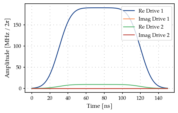
The system consists of two coupled transmons (Koch et al., 2007) [15] with three levels each. We fix the transmon frequency and anharmonicity to values that don’t have any unwanted frequency collisions. The coupling strength is fixed as well. These parameters have to be specified as Quantities with a range, but we will not pass them to the optimizer in order to keep them fixed. Additionally, the first transmon is driven at the frequency of the second one to apply a cross-resonance (CR) gate (Sheldon et al., 2016) [16]. The second transmon is driven to fix the phases of the gate.

Here the tone values are set such that the optimization process is fast. Generally, with a lot of parameters, GOAT (in its current form) can take a considerably long time.

t_final = 150e-9
tone1 = FlatTopGaussianEnvelope(
    amplitude=Quantity(
        190e6 * 2 * np.pi / 2,
        min_value=1e5 * 2 * np.pi,
        max_value=250e6 * 2 * np.pi,
        name="Amp",
        unit="Hz",
        two_pi=True,
    ),
    t_final=Quantity(
        t_final,
        min_value=10e-9,
        max_value=200e-9,
        unit="s",
        name="Gate time",
    ),
)

tone2 = FlatTopGaussianEnvelope(
    amplitude=Quantity(
        9.18e6 * 2 * np.pi / 2,
        min_value=1e5 * 2 * np.pi,
        max_value=250e6 * 2 * np.pi,
        name="Amp",
        unit="Hz",
        two_pi=True,
    ),
    t_final=Quantity(
        t_final,
        min_value=10e-9,
        max_value=200e-9,
        unit="s",
        name="Gate time",
    ),
)


tone2.t_final = Quantity(
    t_final,
    min_value=10e-9,
    max_value=200e-9,
    unit="s",
    name="Gate time",
)

print(tone1.get_parameters(), tone2.get_parameters())
generator1 = IQMixer(
    envelopes=[tone1],
    frequency=Quantity(
        6.0002e9 * 2 * np.pi,
        min_value=5.5e9 * 2 * np.pi,
        max_value=6.20e9 * 2 * np.pi,
        name="Freq",
        unit="Hz",
        two_pi=True,
    ),
)

generator2 = IQMixer(
    envelopes=[tone2],
    frequency=Quantity(
        6.0002e9 * 2 * np.pi,
        min_value=5.5e9 * 2 * np.pi,
        max_value=6.20e9 * 2 * np.pi,
        name="Freq",
        unit="Hz",
        two_pi=True,
    ),
    phase=Quantity(
        value=-0.39720756,
        min_value=-np.pi,
        max_value=np.pi,
        unit="rad",
        name="Phase",
    ),
)


num_levels = 3
transmon_hamiltonian_1 = TransmonHamiltonian(
    num_levels=num_levels,
    frequency=Quantity(
        5.5e9 * 2 * np.pi,
        5.2e9 * 2 * np.pi,
        5.9e9 * 2 * np.pi,
        "Hz",
        "Transmon 1 frequency",
        two_pi=True,
    ),
    anharmonicity=Quantity(
        -240e6 * 2 * np.pi,
        -250e6 * 2 * np.pi,
        -190e6 * 2 * np.pi,
        "Hz",
        "Transmon 1 anharmonicity",
        two_pi=True,
    ),
    drives=[],
)

drive_op1 = transmon_hamiltonian_1.annihilation_op + (transmon_hamiltonian_1.annihilation_op).conj().T
drive1 = Drive(drive_op1, generator1)
transmon_hamiltonian_1.drives = [drive1]

transmon_hamiltonian_2 = TransmonHamiltonian(
    num_levels=num_levels,
    frequency=Quantity(
        6.0e9 * 2 * np.pi,
        5.9e9 * 2 * np.pi,
        6.1e9 * 2 * np.pi,
        "Hz",
        "Transmon 2 frequency",
        two_pi=True,
    ),
    anharmonicity=Quantity(
        -200e6 * 2 * np.pi,
        -210e6 * 2 * np.pi,
        -190e6 * 2 * np.pi,
        "Hz",
        "Transmon 2 anharmonicity",
        two_pi=True,
    ),
    drives=[],
)

drive_op2 = transmon_hamiltonian_2.annihilation_op + (transmon_hamiltonian_2.annihilation_op).conj().T
drive2 = Drive(drive_op2, generator2)
transmon_hamiltonian_2.drives = [drive2]

coupling_op = np.kron(
    transmon_hamiltonian_1.annihilation_op + transmon_hamiltonian_1.annihilation_op.conj().T,
    transmon_hamiltonian_2.annihilation_op + transmon_hamiltonian_2.annihilation_op.conj().T,
)
coupling = Coupling(
    coupling_op,
    g_abs=Quantity(
        25e6 * 2 * np.pi,
        10e6 * 2 * np.pi,
        60e6 * 2 * np.pi,
        "Hz",
        "Coupling strength",
        two_pi=True,
    ),
)
hamiltonian = CompositeHamiltonian([transmon_hamiltonian_1, transmon_hamiltonian_2], [coupling])

[Amp: 95 MHz x 2pi, t_up: 30 ns, t_down: 120 ns, ramp_time: 15 ns] [Amp: 4.59 MHz x 2pi, t_up: 30 ns, t_down: 120 ns, ramp_time: 15 ns]

(transmon_hamiltonian_2.frequency.get_value() - transmon_hamiltonian_1.frequency.get_value()) / (2 * np.pi)

Array([5.e+08], dtype=float64)

from plotting import plot_signal

tlist = np.linspace(0, t_final, 201)
fig, ax = plt.subplots(1, figsize=(5, 3))
plot_signal(tone1, tlist, ax, linestyle="-", label="Drive 1")
plot_signal(tone2, tlist, ax, linestyle="-", label="Drive 2")
ax.legend(loc=1, frameon=True)
plt.show()

We check the eigenvalues to make sure that there is no resonance while idling.

matrix = hamiltonian.get_value(np.array([0.0]))
evals = np.linalg.eigvalsh(matrix)
print("Energies in GHz: ", np.round(evals / 1e6) / 1e3 / (2 * np.pi))
transitions = evals[1:] - evals[:-1]
print(
    "Transition energies in GHz: ",
    np.round(transitions / 1e3) / 1e6 / (2 * np.pi),
)
matrix

Energies in GHz:  [[-0.          5.49864413  6.00109628 10.75823753 11.49735309 11.80404466 16.7555141  17.30475781 22.56021318]]
Transition energies in GHz:  []

Array([[[0.00000000e+00+0.j, 6.22009913e+04+0.j, 0.00000000e+00+0.j, 1.39607610e+06+0.j, 1.57079633e+08+0.j, 0.00000000e+00+0.j, 0.00000000e+00+0.j, 0.00000000e+00+0.j, 0.00000000e+00+0.j],
        [6.22009913e+04+0.j, 3.76991118e+10+0.j, 8.79654856e+04+0.j, 1.57079633e+08+0.j, 1.39607610e+06+0.j, 2.22144147e+08+0.j, 0.00000000e+00+0.j, 0.00000000e+00+0.j, 0.00000000e+00+0.j],
        [0.00000000e+00+0.j, 8.79654856e+04+0.j, 7.41415866e+10+0.j, 0.00000000e+00+0.j, 2.22144147e+08+0.j, 1.39607610e+06+0.j, 0.00000000e+00+0.j, 0.00000000e+00+0.j, 0.00000000e+00+0.j],
        [1.39607610e+06+0.j, 1.57079633e+08+0.j, 0.00000000e+00+0.j, 3.45575192e+10+0.j, 6.22009913e+04+0.j, 0.00000000e+00+0.j, 1.97434975e+06+0.j, 2.22144147e+08+0.j, 0.00000000e+00+0.j],
        [1.57079633e+08+0.j, 1.39607610e+06+0.j, 2.22144147e+08+0.j, 6.22009913e+04+0.j, 7.22566310e+10+0.j, 8.79654856e+04+0.j, 2.22144147e+08+0.j, 1.97434975e+06+0.j, 3.14159265e+08+0.j],
        [0.00000000e+00+0.j, 2.22144147e+08+0.j, 1.39607610e+06+0.j, 0.00000000e+00+0.j, 8.79654856e+04+0.j, 1.08699106e+11+0.j, 0.00000000e+00+0.j, 3.14159265e+08+0.j, 1.97434975e+06+0.j],
        [0.00000000e+00+0.j, 0.00000000e+00+0.j, 0.00000000e+00+0.j, 1.97434975e+06+0.j, 2.22144147e+08+0.j, 0.00000000e+00+0.j, 6.76070739e+10+0.j, 6.22009913e+04+0.j, 0.00000000e+00+0.j],
        [0.00000000e+00+0.j, 0.00000000e+00+0.j, 0.00000000e+00+0.j, 2.22144147e+08+0.j, 1.97434975e+06+0.j, 3.14159265e+08+0.j, 6.22009913e+04+0.j, 1.05306186e+11+0.j, 8.79654856e+04+0.j],
        [0.00000000e+00+0.j, 0.00000000e+00+0.j, 0.00000000e+00+0.j, 0.00000000e+00+0.j, 3.14159265e+08+0.j, 1.97434975e+06+0.j, 0.00000000e+00+0.j, 8.79654856e+04+0.j, 1.41748661e+11+0.j]]], dtype=complex128)

Computing the gate fidelity

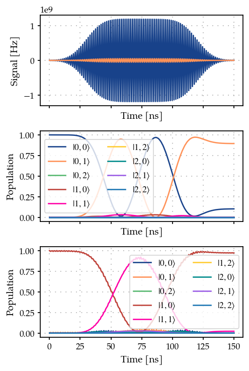
We select a propagation method, piecewise constant exponentiation, and configure CR as a target gate.

model = SchroedingerEquation(
    hamiltonian_func=hamiltonian.get_value,
    hamiltonian_gradient_func=hamiltonian.get_gradient,
)

# We need to pad the operators with zeros so we introduce a helper zero matrix
dim = transmon_hamiltonian_1.dimension() * transmon_hamiltonian_2.dimension()
padding = ((0, dim - 4), (0, dim - 4))

sigma_x = sigma_x()
sigma_y = sigma_y()
sigma_z = sigma_z()

pauli_ix = np.pad(np.kron(np.identity(2), sigma_x), pad_width=padding, mode="constant", constant_values=0.0)
pauli_iy = np.pad(np.kron(np.identity(2), sigma_y), pad_width=padding, mode="constant", constant_values=0.0)
pauli_iz = np.pad(np.kron(np.identity(2), sigma_z), pad_width=padding, mode="constant", constant_values=0.0)

pauli_zx = np.pad(
    np.exp(1j * np.pi / 4) * np.kron(sigma_z, sigma_x), pad_width=padding, mode="constant", constant_values=0.0
)

cr_gate = np.pad(
    np.array([[1.0, 0, 0, 0], [0, 1.0, 0, 0], [0, 0, 0, 1.0], [0, 0, 1.0, 0]]),
    pad_width=padding,
    mode="constant",
    constant_values=0.0,
)

cr_gate = pauli_zx @ cr_gate

times = np.array([0.0, t_final])

prop = GOAT(
    Expm(
        eom_func=model.get_value,
        resolution=100e9,
        initial_state=np.identity(transmon_hamiltonian_1.dimension() * transmon_hamiltonian_2.dimension()),
    ),
    eom_gradient_func=model.get_gradient,
)

gate_fid = UnitaryFidelity(
    propagation_func=prop.get_value,
    propagation_gradient_func=prop.get_gradient,
    gate=cr_gate,
)
gate_fid.get_value(times)

Array(0.03713341, dtype=float64)

def plot_population(propagation: Propagation):
    """Plot the population from the Propagation object."""
    basis1 = [i for i in range(transmon_hamiltonian_1.dimension())]
    basis2 = [i for i in range(transmon_hamiltonian_2.dimension())]
    labels = [rf"$|{i},{j}\rangle$" for (i, j) in itertools.product(basis1, basis2)]

    signal1 = generator1.get_value(tlist)
    signal2 = generator2.get_value(tlist)
    states = propagation.get_value(tlist)

    _, ax = plt.subplots(3, figsize=(4, 6), sharex=True)
    ax[0].plot(tlist / 1e-9, signal1)
    ax[0].plot(tlist / 1e-9, signal2)
    ax[0].set_xlabel("Time [ns]")
    ax[0].set_ylabel("Signal [Hz]")
    ax[0].grid(True, linestyle=(1, (1, 5)), linewidth=1)

    ax[1].plot(tlist / 1e-9, np.abs(states)[:, :, 0] ** 2, label=labels)
    ax[1].set_xlabel("Time [ns]")
    ax[1].set_ylabel("Population")
    ax[1].legend(ncols=2)
    ax[1].grid(True, linestyle=(1, (1, 5)), linewidth=1)

    ax[2].plot(
        tlist / 1e-9,
        np.abs(states)[:, :, transmon_hamiltonian_2.dimension()] ** 2,
        label=labels,
    )
    ax[2].set_xlabel("Time [ns]")
    ax[2].set_ylabel("Population")
    ax[2].legend(ncols=2)
    ax[2].grid(True, linestyle=(1, (1, 5)), linewidth=1)

    plt.tight_layout()
    plt.show()


plot_population(prop)

def expecation_value(Op, states):
    """Get the expected value."""
    ex = []
    for state in states:
        ex.append(np.real(state.conj() @ Op @ state.T))
    return ex


def plot_pauli():
    """Plot the Pauli operators."""
    states = prop.get_value(tlist)
    sig1 = generator1.get_value(tlist)
    sig2 = generator2.get_value(tlist)

    fig, ax = plt.subplots(3, figsize=(4, 6), sharex=True)
    ax[0].plot(tlist / 1e-9, sig1)
    ax[0].plot(tlist / 1e-9, sig2)
    ax[0].set_ylabel("Field [MHz]")
    ax[0].grid(True, linestyle=(1, (1, 5)), linewidth=1)

    ax[1].plot(tlist / 1e-9, expecation_value(pauli_ix, states[:, :, 0]))
    ax[1].plot(tlist / 1e-9, expecation_value(pauli_iy, states[:, :, 0]))
    ax[1].plot(tlist / 1e-9, expecation_value(pauli_iz, states[:, :, 0]))
    ax[1].set_ylabel(r"$\langle 0, x|\hat\sigma_i|0, x\rangle$")
    ax[1].legend(["X", "Y", "Z"])
    ax[1].grid(True, linestyle=(1, (1, 5)), linewidth=1)

    ax[2].plot(tlist / 1e-9, expecation_value(pauli_ix, states[:, :, transmon_hamiltonian_2.dimension()]))
    ax[2].plot(tlist / 1e-9, expecation_value(pauli_iy, states[:, :, transmon_hamiltonian_2.dimension()]))
    ax[2].plot(tlist / 1e-9, expecation_value(pauli_iz, states[:, :, transmon_hamiltonian_2.dimension()]))
    ax[2].set_ylabel(r"$\langle 1, x|\hat\sigma_i|1, x\rangle$")
    ax[-1].set_xlabel("Time [ns]")
    ax[2].legend(["X", "Y", "Z"])
    ax[2].grid(True, linestyle=(1, (1, 5)), linewidth=1)
    plt.show()


plot_pauli()

Optimization

We define an optimizer and link our fidelity measure as a goal function. The only optimizable parameter is the frequency of transmon 1.

tone1.get_parameters()

[Amp: 95 MHz x 2pi, t_up: 30 ns, t_down: 120 ns, ramp_time: 15 ns]

optmap = OptimizationMap()
optmap.add(tone1)
print(optmap)

opt = ScipyOptimizerGradient(measure_and_gradient_func=gate_fid.get_value_and_gradient, optimization_map=optmap)
opt.set_options({"ftol": 0.1, "maxls": 50, "gtol": 1e-8})

==== <class 'paraqeet.signal.envelopes.FlatTopGaussianEnvelope'> ====
[Amp: 95 MHz x 2pi, t_up: 30 ns, t_down: 120 ns, ramp_time: 15 ns]

optmap

==== <class 'paraqeet.signal.envelopes.FlatTopGaussianEnvelope'> ====
[Amp: 95 MHz x 2pi, t_up: 30 ns, t_down: 120 ns, ramp_time: 15 ns]

opt.optimize(times)

{'status': 1, 'value': 0.9362484996671709, 'iterations': 2, 'message': 'CONVERGENCE: RELATIVE REDUCTION OF F <= FACTR*EPSMCH'}

plot_population(prop)

plot_pauli()

References

• (Koch et al., 2007) J. Koch et al., “Charge-insensitive qubit design derived from the Cooper pair box,” Physical Review A 76, 042319 (2007).

• (Sheldon et al., 2016) S. Sheldon et al., “Procedure for systematically tuning up cross-talk in the cross-resonance gate,” Physical Review A 93, 060302 (2016).