Gradient based dCRAB optimization of a single spin#
In this example, we solve the optimization task in the previous example by using the dCRAB optimization method. Here we implement a gradient based dCRAB algorithm by using the GOAToverGRAPE method.
1. Generate a PWC pulse shape#
import jax.numpy as jnp
import matplotlib.pyplot as plt
import numpy as np

from paraqeet.quantity import Quantity
from paraqeet.signal.envelopes import DCRABEnvelope
from paraqeet.signal.pwc_generator import PWCGenerator
from paraqeet.signal.waveform import FlatTopGaussianFilter
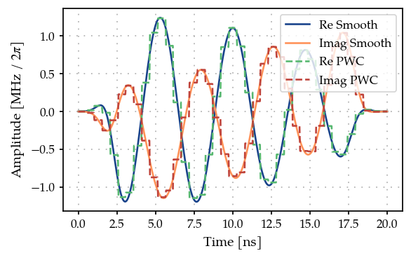
Similar to the previous case, lets define the pulse generator, with the
envelope being the DCRABEnvelope. We use a FlatTopGaussianFilter
to ensure that the pulse always starts and ends at zero. Finally, to
obtain GRAPE gradient we pixelate the pulse using a PWCGenerator.
t_final = 20e-9
tlist = np.linspace(0, t_final, 40)
eps = 5 * np.pi * 1.0  # initial amplitude of the resonator (in MHz)
eps_max = 10 * eps  # maximum amplitude of the resonator (in MHz)

tone = DCRABEnvelope(
    num_components=2,
    max_frequency=5 * 2 * np.pi,
    amplitude=Quantity(eps * 1e6, -eps_max * 1e6, eps_max * 1e6, name="Amplitude"),
    t_final=Quantity(t_final, 1 / 2 * t_final, 2 * t_final, name="t_final"),
    seed=18537,
)
smooth_tone = FlatTopGaussianFilter(
    envelopes=tone, t_final=Quantity(t_final, 1 / 2 * t_final, 2 * t_final, name="t_final")
)

gen = PWCGenerator(envelopes=[smooth_tone], tlist=tlist, max_amplitude=np.sqrt(2) * eps_max * 1e6)

params = gen.get_parameters()
Here the DCRABEnvelope is defined with a seed to make sure that the
results obtained are reproducible.
from plotting import plot_signal

ts = np.linspace(0, t_final, 501)
fig, ax = plt.subplots(1, figsize=(5, 3))
plot_signal(smooth_tone, ts, ax, linestyle="-", label="Smooth")
plot_signal(gen, ts, ax, linestyle="--", label="PWC")
ax.legend(loc=1, frameon=True)
plt.show()
2. Define Hamiltonian in the rotating frame of drive#
As before we define a single spin in the rotating frame of the drive.
from paraqeet.model.closed_system import ClosedSystem
from paraqeet.model.differentiable_hamiltonian import DifferentiableHamiltonian
from paraqeet.model.rotating_frame_drive import RotatingFrameDrive
from paraqeet.quantity import Array


class SpinRWA(DifferentiableHamiltonian):
    """A Single Spin."""

    def __init__(self, drives=None):
        super().__init__(drives)
        self.sigma_p = jnp.array([[0j, 1], [0, 0]])
        self.dim = 2

    def get_value_at_timestep(self, timestep: float) -> Array:
        """Just sigma-X."""
        return self._drives[0].get_value_at_timestep(self.sigma_p, timestep)

    def get_value_and_gradient(self, times: Array) -> tuple[Array, Array] | tuple[float, Array]:
        """Gradient is just the drive matrix."""
        return self.get_value(times), self._drives[0].get_gradient(self.sigma_p, times)

    def get_gradient_at_timestep(self, time):
        """Computes the gradient"""
        return self._drives[0].get_gradient_at_timestep(self.sigma_p, time)

    def dimension(self) -> int:
        """Returns the dimension"""
        raise self.d

    def get_collapseops(self) -> list[tuple[Array, Array]]:
        """Returns an empyt list since we study closed system dynamics"""
        return []

    def get_parameters(self):
        """Returns the parameters, which in this case are only the drive parameters"""
        return self._get_drive_parameters()


drive = RotatingFrameDrive(gen)
spin = SpinRWA(drives=[drive])
model = ClosedSystem(spin)
And using GRAPE as the method to propagate and compute the gradients. The propagation \(dt\) has to be smaller than the \(\Delta t\) of the time grid used for discretization. In this case \(\Delta t = 0.5\) ns, so we choose the propagation resolution to be > 2e9.
from paraqeet.measurement.state_transfer_fidelity import StateTransferFidelityGRAPE
from paraqeet.propagation.scipy_expm_grape import ScipyExpmGRAPE

prop = ScipyExpmGRAPE(model, resolution=3e9)

init = np.array([[1.0], [0]])  # |0>
target = np.array([[0.0], [1]])  # |1>

prop.set_initial_state(init)
prop.set_target_state(target)

zeroone = StateTransferFidelityGRAPE(
    propagation=prop,
    initial_state=init,
    target_state=target,
)
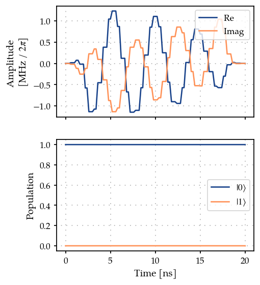
from plotting import plot_signal_and_dynamics

ts = np.linspace(0.0, t_final, 101)
plot_signal_and_dynamics(gen, prop, ts, state_labels=[r"$|0\rangle$", r"$|1\rangle$"]);
3. Optimisation#
Finally, we define the DCRABOptimizerGradient that takes the
GOATOverGRAPE fideltiy to chains together the GRAPE gradients to
compute the gradient wrt the dCRAB envelope
params = tone.get_parameters()
params
[Amplitude: 1.57e+07,
 t_final: 2e-08,
 CRAB Re coefficient 0: 0.801,
 CRAB Re coefficient 1: -0.707,
 CRAB Re frequency 0: 4 Hz x 2pi,
 CRAB Re frequency 1: 4.51 Hz x 2pi,
 CRAB Re Phase 0: -75.6 mHz x 2pi,
 CRAB Re Phase 1: 320 mHz x 2pi,
 CRAB Im coefficient 0: -0.419,
 CRAB Im coefficient 1: 0.72,
 CRAB Im frequency 0: 472 mHz x 2pi,
 CRAB Im frequency 1: 4.27 Hz x 2pi,
 CRAB Im Phase 0: -23.1 mHz x 2pi,
 CRAB Im Phase 1: 317 mHz x 2pi]
Here we add the parameters from the DCRABEnvelope to the optmap
(except the t_final to keep the simulation time constant)
import tempfile

from paraqeet.file_logger import FileLogger
from paraqeet.measurement.goat_over_grape import GOATOverGRAPE
from paraqeet.optimization_map import OptimizationMap
from paraqeet.optimizers.dcrab_optimizer_gradient import DCRABOptimizerGradient

temp_dir = tempfile.TemporaryDirectory()

file_logger = FileLogger(temp_dir.name)

optmap = OptimizationMap()
optmap.add(tone, [params[0]] + params[2:])
optmap.register_params_with_optimizables()

goat = GOATOverGRAPE(zeroone, prop, generators=[gen])
opt_grad = DCRABOptimizerGradient(
    goat,
    optimization_map=optmap,
    super_iteration_every=150,
    max_super_iteration_num=5,
    print_every_iteration_num=10,
    super_iteration_tol=1e-9,
    seed=19573,
)
opt_grad.logger = file_logger
The optmap in this case contains the pulse amplitude and the Fourier
coefficients for the optimization.
optmap
==== <class 'paraqeet.signal.envelopes.DCRABEnvelope'> ====
[Amplitude: 1.57e+07, CRAB Re coefficient 0: 0.801, CRAB Re coefficient 1: -0.707, CRAB Re frequency 0: 4 Hz x 2pi, CRAB Re frequency 1: 4.51 Hz x 2pi, CRAB Re Phase 0: -75.6 mHz x 2pi, CRAB Re Phase 1: 320 mHz x 2pi, CRAB Im coefficient 0: -0.419, CRAB Im coefficient 1: 0.72, CRAB Im frequency 0: 472 mHz x 2pi, CRAB Im frequency 1: 4.27 Hz x 2pi, CRAB Im Phase 0: -23.1 mHz x 2pi, CRAB Im Phase 1: 317 mHz x 2pi]
opt_grad.optimize(np.array([0.0, t_final]))
scipy.optimize: The disp and iprint options of the L-BFGS-B solver are deprecated and will be removed in SciPy 1.18.0.
Iteration number = 0 Infidelity = 9.999e-01
Iteration number = 10 Infidelity = 3.178e-05
Setting parameters to the best values.
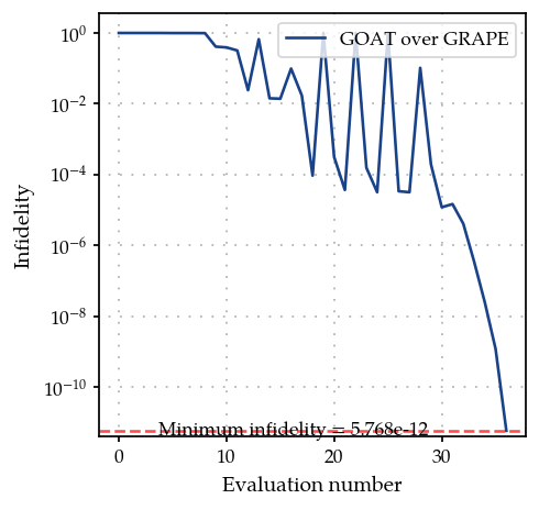
{'status': 1, 'value': 5.767608612927688e-12, 'iterations': 37, 'message': 'CONVERGENCE: NORM OF PROJECTED GRADIENT <= PGTOL'}
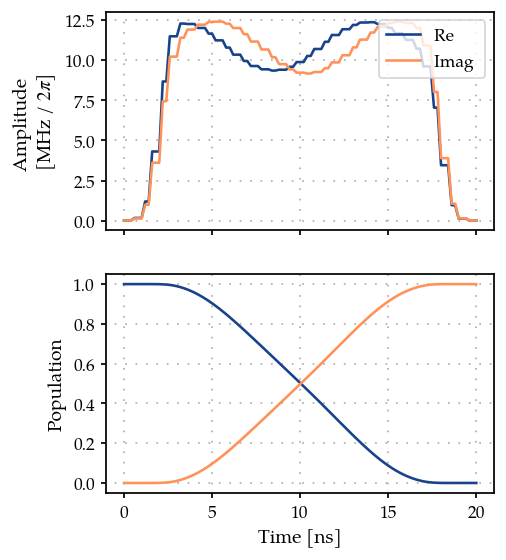
As the parameters are added with random values, the optimization may not succeed sometimes. If it does not reach a low value restart the optimization. Here, we have chosen a seed that converges to the target fidelity.
opt_grad.set_parameters(opt_grad.best_params)
plot_signal_and_dynamics(gen, prop, ts);
from plotting import plot_infidelity_vs_evaluation_from_logs

plot_infidelity_vs_evaluation_from_logs(log_path=temp_dir.name + "/opt.log", label="GOAT over GRAPE");
temp_dir.cleanup()