

GRAPE on a single spin#
This is an introductory example to the GRAPE (Khaneja et al., 2005) [1] method and its implementation in this software package.
1. Generate a PWC pulse shape#
import matplotlib.pyplot as plt
import numpy as np

from paraqeet.eom.schroedinger_equation import SchroedingerEquation
from paraqeet.hamiltonian.drive import Drive
from paraqeet.hamiltonian.qubit import QubitHamiltonian
from paraqeet.quantity import Quantity
from paraqeet.signal.envelopes import GaussEnvelope
from paraqeet.signal.pwc_generator import PWCGenerator
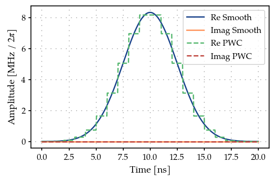
First, let’s generate a piecewise constant (PWC) pulse envelope for the Gaussian pulse. For GRAPE, we need to specify an ansatz for piecewise constant controls at a given resolution. Here, we set up a Gaussian initial guess, sampling at 21 points during a gate time of 20 ns.
t_final = 20e-9
tlist = np.linspace(0, t_final, 21)
tone = GaussEnvelope(amplitude=Quantity(np.pi / t_final / 3, -np.pi / t_final, np.pi / t_final))
tone.t_final.set_value(t_final)

gen = PWCGenerator(envelopes=[tone], tlist=tlist)
gen.multiply_flat_top = True
gen.max_amplitude = 2 * 1e8
We have added the option multiply_flat_top, to ensure the pulse
starts and ends smoothly at 0 and t_final. This acts like the
FlatTopGaussianFilter, but enforced directly by the
PWCGenerator.
from plotting import plot_signal

ts = np.linspace(0, t_final, 501)
fig, ax = plt.subplots(1, figsize=(5, 3))
plot_signal(tone, ts, ax, linestyle="-", label="Smooth")
plot_signal(gen, ts, ax, linestyle="--", label="PWC")
ax.legend(loc=1, frameon=True)
plt.show()
2. Define Hamiltonian in the rotating frame of drive#
As a simple toy model, we use a single spin.
qubit_hamiltonian = QubitHamiltonian(frequency=Quantity(0.0, 0.0, 2 * np.pi * 1e6, unit="Hz"), drives=[])
drive = Drive(qubit_hamiltonian.sigma_minus, gen, add_hermitian=True)
qubit_hamiltonian.drives = [drive]
model = SchroedingerEquation(
    hamiltonian_func=qubit_hamiltonian.get_value,
    hamiltonian_gradient_func=qubit_hamiltonian.get_gradient,
)
from paraqeet.measurement.state_transfer_fidelity import StateTransferFidelityGRAPE
from paraqeet.measurement.utils import overlap_state_vector
from paraqeet.propagation import GRAPE, Expm
from paraqeet.propagation.utils import grape_operator_sandwich_function_closed

init = np.array([[1.0], [0.0]])  # |0>
target = np.array([[0.0], [1.0]])  # |1>

propagation = Expm(eom_func=model.get_value, resolution=2e9, initial_state=init)
prop = GRAPE(
    propagation,
    eom_gradient_func=model.get_gradient,
    target_state=target,
    operator_sandwich_function=grape_operator_sandwich_function_closed,
    order=3
)

times = np.array([0.0, t_final])

zeroone = StateTransferFidelityGRAPE(
    propagation_func=prop.get_value,
    propagation_gradient_func=prop.get_gradient,
    target_state=target,
    overlap=overlap_state_vector,
)
from plotting import plot_signal_and_dynamics

ts = np.linspace(0.0, t_final, 101)
plot_signal_and_dynamics(gen, prop, ts, state_labels=[r"$|0\rangle$", r"$|1\rangle$"])
array([<Axes: ylabel='Amplitude n[MHz / $2\pi$]'>,
       <Axes: xlabel='Time [ns]', ylabel='Population'>], dtype=object)

zeroone.get_value(times)
Array(0.10336679, dtype=float64)
from paraqeet.optimization_map import OptimizationMap
from paraqeet.optimizers.scipy_optimizer_gradient import ScipyOptimizerGradient

optmap = OptimizationMap()
optmap.add(gen)
optmap.register_params_with_optimizables()

opt_grad = ScipyOptimizerGradient(measure_and_gradient_func=zeroone.get_value_and_gradient, optimization_map=optmap)
Unlike the previous examples, for GRAPE based optimization, we need to
specify the exact time grid used to discretize the signal for
optimization. This is required to compute the correct gradients at the
exact time points. The time grid used for discretization can be found
from a PWCGenerator using gen.tlist.
opt_grad.optimize(gen.tlist)
{'status': 1, 'value': 3.647304680498564e-11, 'iterations': 20, 'message': 'CONVERGENCE: RELATIVE REDUCTION OF F <= FACTR*EPSMCH'}
For this simple example, we reach near-perfect fidelity within a few iterations.
plot_signal_and_dynamics(gen, prop, ts, state_labels=[r"$|0\rangle$", r"$|1\rangle$"])
array([<Axes: ylabel='Amplitude n[MHz / $2\pi$]'>,
       <Axes: xlabel='Time [ns]', ylabel='Population'>], dtype=object)

With open system#
Let’s first reset the pulse and create an open-system model
import numpy as np

from paraqeet.quantity import Quantity
from paraqeet.signal.envelopes import GaussEnvelope
from paraqeet.signal.pwc_generator import PWCGenerator
tone = GaussEnvelope(amplitude=Quantity(np.pi / t_final / 3, -np.pi / t_final, np.pi / t_final))
tone.t_final.set_value(t_final)
gen = PWCGenerator(envelopes=[tone], tlist=tlist)
gen.multiply_flat_top = True
gen.max_amplitude = 5 * 1e8
import jax.numpy as jnp

from paraqeet.eom.master_equation import MasterEquation
from paraqeet.hamiltonian.qubit import Qubit

t1 = Quantity(10e-6, 1e-6, 100e-6)
temp = Quantity(10e-3, 1e-3, 50e-3)
t2star = Quantity(20e-6, 1e-6, 100e-6)


qubit_hamiltonian = QubitHamiltonian(frequency=Quantity(0.0, 0.0, 2 * np.pi * 1e6, unit="Hz"), drives=[])
drive = Drive(qubit_hamiltonian.sigma_minus, gen, add_hermitian=True)
qubit_hamiltonian.drives = [drive]

open_qubit = Qubit(hamiltonian=qubit_hamiltonian, t1=t1, temp=temp, t2star=t2star)

model = MasterEquation(
    hamiltonian_func=qubit_hamiltonian.get_value,
    hamiltonian_gradient_func=qubit_hamiltonian.get_gradient,
    jump_operators=open_qubit.get_jump_operators(),
)
Let’s test GRAPE with ODE propagation
from paraqeet.measurement.state_transfer_fidelity import StateTransferFidelityGRAPE
from paraqeet.measurement.utils import overlap_density_matrix
from paraqeet.propagation import GRAPE, Vern7
from paraqeet.propagation.utils import grape_operator_sandwich_function_open, lindblad_step, reverse_lindblad_step

init = np.array([[1.0], [0.0j]])  # |0>
target = np.array([[0.0j], [1.0]])  # |1>

init = jnp.matmul(init, init.T.conj())
target = jnp.matmul(target, target.T.conj())

propagation = Vern7(
    eom_func=model.get_eom_ode_propagation,
    resolution=10e9,
    initial_state=init,
    step_function=lindblad_step,
    jump_operators=open_qubit.get_jump_operators(),
)
# The dissipator is built from the collapse operators inside the step function rather than being
# part of the equation of motion, so the backward propagation needs the adjoint dissipator.
prop = GRAPE(
    propagation,
    eom_gradient_func=model.get_eom_gradient_ode_propagation,
    target_state=target,
    operator_sandwich_function=grape_operator_sandwich_function_open,
    reverse_step_function=reverse_lindblad_step,
    order=3
)

zeroone = StateTransferFidelityGRAPE(
    propagation_func=prop.get_value,
    propagation_gradient_func=prop.get_gradient,
    target_state=target,
    overlap=overlap_density_matrix,
)
init
Array([[1.+0.j, 0.+0.j],
       [0.+0.j, 0.+0.j]], dtype=complex128)
ts = np.linspace(0, t_final, 101)
plot_signal_and_dynamics(gen, prop, times=ts, state_labels=[r"$\rho_0$", r"$\rho_1$"], open_system=True)
array([<Axes: ylabel='Amplitude n[MHz / $2\pi$]'>,
       <Axes: xlabel='Time [ns]', ylabel='Population'>], dtype=object)

zeroone.get_value(times)
Array(0.0109956, dtype=float64)
from paraqeet.optimization_map import OptimizationMap
from paraqeet.optimizers.scipy_optimizer_gradient import ScipyOptimizerGradient

optmap = OptimizationMap()
optmap.add(gen)
optmap.register_params_with_optimizables()
opt_grad = ScipyOptimizerGradient(measure_and_gradient_func=zeroone.get_value_and_gradient, optimization_map=optmap)
opt_grad.optimize(tlist)
{'status': 2, 'value': 0.005283974963344429, 'iterations': 54, 'message': 'ABNORMAL: '}
plot_signal_and_dynamics(gen, prop, times=ts, state_labels=[r"$\rho_0$", r"$\rho_1$"], open_system=True)
array([<Axes: ylabel='Amplitude n[MHz / $2\pi$]'>,
       <Axes: xlabel='Time [ns]', ylabel='Population'>], dtype=object)

zeroone.get_value(times)
Array(0.99471603, dtype=float64)
References#
(Khaneja et al., 2005) N. Khaneja et al., “Optimal control of coupled spin dynamics: design of NMR pulse sequences by gradient ascent algorithms,” Journal of Magnetic Resonance 172, 296–305 (2005).