DRAG Correction of a Gaussian Pulse#
First, we make the necessary imports.
import numpy as np

from paraqeet.measurement.unitary_fidelity import UnitaryFidelity
from paraqeet.model.closed_system import ClosedSystem
from paraqeet.model.drive_operator import DriveOperator
from paraqeet.model.transmon import Transmon
from paraqeet.optimization_map import OptimizationMap
from paraqeet.optimizers.scipy_optimizer import ScipyOptimizer
from paraqeet.propagation.scipy_expm_goat import ScipyExpmGOAT
from paraqeet.quantity import Quantity
from paraqeet.signal.envelopes import GaussEnvelope
from paraqeet.signal.iq_mixer import IQMixer
from paraqeet.signal.waveform import DRAGMixer
1. Define the Gaussian Tone and put into the DRAGMixer#
The GaussTone explicitly allows for the evaluation of an envelope signal and its time derivative which is then used to calculate the DRAG corrected signal in the DRAGMixer
t_final = 20e-9
env_tone = GaussEnvelope()
env_tone.t_final.set_value(t_final)
drag_tone = DRAGMixer(envelopes=env_tone)
drag_tone._envs[0]._delta
Delta: -1.26 GHz
gen = IQMixer(envelopes=[drag_tone])
freq = 4.8e9 * 2 * np.pi
anhar = -200e6 * 2 * np.pi

qubit_levels = 3

drive = DriveOperator(gen, is_longitudinal=False)
controlled_transmon = Transmon(
    frequency=Quantity(
        freq,
        min_value=np.array(freq / 4),
        max_value=np.array(freq * 1.2),
        unit="Hz",
        name="Qubit frequency",
    ),
    anharmonicity=Quantity(
        anhar,
        min_value=np.array(anhar * 1.2),
        max_value=np.array(anhar * 0.8),
        unit="Hz",
        name="Qubit anharmonicity",
    ),
    dimension=qubit_levels,
    drives=[drive],
)

model = ClosedSystem(controlled_transmon)

params = gen.get_parameters()

prop = ScipyExpmGOAT(model, resolution=500e9)
prop.set_initial_state(np.eye(qubit_levels))
params
[Amplitude: 24.7 MHz x 2pi,
 t_final: 20 ns,
 Delta: -1.26 GHz,
 lo_freq: 4.8 GHz x 2pi,
 Phase: 0 rad]
params[0].set_value(3e8)
params[2].set_value(2 * anhar)
gen.get_parameters()
[Amplitude: 47.7 MHz x 2pi,
 t_final: 20 ns,
 Delta: -2.51 GHz,
 lo_freq: 4.8 GHz x 2pi,
 Phase: 0 rad]
2. Set up ideal reference matrix to compare the pulses result to.#
def rx(theta) -> np.ndarray:
    """Get the ideal representation of a rx rotation of angle theta."""
    return np.array(
        [
            [np.cos(theta / 2), -1j * np.sin(theta / 2), 0],
            [-1j * np.sin(theta / 2), np.cos(theta / 2), 0],
            [0, 0, 1],
        ],
        dtype=np.complex128,
    )
Set up measure that is optimized. In this case, the gate fidelity between the propagator resulting from the pulse simulation and the ideal reference defined above is used.
gate_fid = UnitaryFidelity(
    propagation=prop,
    gate=rx(np.pi / 2),
)
Plot initial pulse shape and population transfer. Target is the full population transfer,i.e., an X-gate.
from plotting import plot_signal_and_dynamics

ts = np.linspace(0.0, t_final, 1001)
plot_signal_and_dynamics(gen, prop, ts, state_labels=[r"$|0\rangle$", r"$|1\rangle$"]);
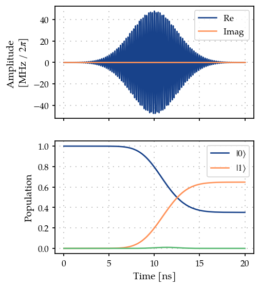
As expected, we get a partial transfer and a low fidelity.
times = np.array([0.0, t_final])
gate_fid.measure(times)
0.9729714831357765
3. Optimization#
We define an optimizer and link our fidelity measure as a goal function and the parameters of the cosine tone.
optmap = OptimizationMap()
selected_params = []
for i in [0, 2, 3, 4]:
    selected_params.append(params[i])
optmap.add(gen, selected_params)
opt = ScipyOptimizer(gate_fid, optimization_map=optmap)
opt.optimize(times)
{'status': 1, 'value': 0.005761021428613344, 'iterations': 90, 'message': 'CONVERGENCE: RELATIVE REDUCTION OF F <= FACTR*EPSMCH'}
Print all parameters that were optimized.
print("{: >15}: {: >20} {: >20} {: >20}".format("Name", "Value", "Min", "Max"))
print("-" * 80)
for par in selected_params:
    print(
        f"{par.get_name(): >15}: {par.get_value()[0]: >20.6e} "
        f"{par.get_min_value()[0]: >20.6e} {par.get_max_value()[0]: >20.6e}"
    )
           Name:                Value                  Min                  Max
--------------------------------------------------------------------------------
      Amplitude:         2.446315e+08         0.000000e+00         1.000000e+09
          Delta:        -2.495595e+09        -3.769911e+09        -1.256637e+08
        lo_freq:         3.015945e+10         2.412743e+10         3.619115e+10
          Phase:         1.380402e-03        -3.141593e+00         3.141593e+00
Plot final pulse shape and population transfer. Target is the full population transfer,i.e., an X-gate.
plot_signal_and_dynamics(gen, prop, ts, state_labels=[r"$|0\rangle$", r"$|1\rangle$"]);
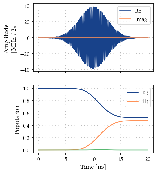
We can see from the plot and optimizer output that we have found better controls. For which the excitement to the second excited state is much smaller than initially.
gate_fid.measure(times)
0.9942389785757956