State preparation of a single spin

In this notebook, we will study a simple problem of state preparation for a single spin or qubit.

import numpy as np

from paraqeet.measurement.state_transfer_fidelity import StateTransferFidelity
from paraqeet.model.closed_system import ClosedSystem
from paraqeet.model.drive_operator import DriveOperator
from paraqeet.model.qubit import Qubit
from paraqeet.optimization_map import OptimizationMap
from paraqeet.optimizers.scipy_optimizer import ScipyOptimizer
from paraqeet.propagation.scipy_expm import ScipyExpm
from paraqeet.quantity import Quantity
from paraqeet.signal.envelopes import ConstantEnvelope
from paraqeet.signal.iq_mixer import IQMixer

System Setup

We first set up the qubit system we want to control. We set the qubit frequency \(\omega_q / 2 \pi\) to be \(4.8\) GHz and define the Hamiltonian as

\[H(t)=H_\text{drift}+H_c(t)= \frac{\omega_q}{2} \sigma_z + \Omega(t)\sigma_x,\]

where \(\Omega(t)\) will be supplied by the generator.

freq_q = 4.8e9
omega_q = 2 * np.pi * freq_q

controlled_qubit = Qubit(frequency=Quantity(omega_q, 0.8 * omega_q, 1.2 * omega_q, unit="Hz", two_pi=True), drives=[])
model = ClosedSystem(controlled_qubit)

For signal generation, we define a simple cosine shaped tone generator \(A \cos(\omega t)\)

tone = ConstantEnvelope()
gen = IQMixer(envelopes=[tone])

We can inspect the pre-defined parameters with

params_tone = tone.get_parameters()
print(params_tone)
params_gen = gen.get_parameters()
print(params_gen)

[Amplitude: 24.7 MHz x 2pi, t_final: 32 ns]
[Amplitude: 24.7 MHz x 2pi, t_final: 32 ns, lo_freq: 4.8 GHz x 2pi, Phase: 0 rad]

In this notebook, we would like to optimize the amplitude Amplitude and frequency lo_freq if the drive. We add a drive on the qubit.

drive = DriveOperator(gen, is_longitudinal=False)
controlled_qubit.drives = [drive]
model = ClosedSystem(controlled_qubit)

Textbook values for implementing an \(X\) rotation on this system at a time \(T\) would be \(\omega=\omega_q\) and \(A=\pi/T\). We use some offset from these values as initial guess to demonstrate the optimization procedure.

t_simu = 10e-9
params_gen[0].set_value(0.8 * np.pi / t_simu)
params_gen[2].set_value(1.01 * omega_q)

It is important to note that, although we changed the parameters of params_gen the corresponding parameter of params_tone also changes, due Python’s “Pass By Object Reference” scheme. In fact,

print(params_tone)
print(params_gen)

[Amplitude: 40 MHz x 2pi, t_final: 32 ns]
[Amplitude: 40 MHz x 2pi, t_final: 32 ns, lo_freq: 4.85 GHz x 2pi, Phase: 0 rad]

We can try to see what happens if we print the gradient of the controlled qubit at the time t_simu:

print(controlled_qubit.get_gradient_at_timestep(np.array([t_simu])))

[]

We see that in this case it is empty. This is because, we haven’t yet defined an OptimizationMap object that defines the optimizable parameters. Also note that the tone parameter t_final is simply the time after which the pulse it is assumed to be zero and it is set by default to \(32 \, \mathrm{ns}\). This is not necessarily the simulation time, which is another parameter of our choice called t_simu in this case.

Next, we select a propagation method, piecewise constant exponentiation, and configure a state transfer problem from \(\ket{0}\) to \(\ket{1}\).

prop = ScipyExpm(model, resolution=100e9)  # implicit timestep is 1 / resolution
times = np.array([0.0, t_simu])


init = np.array([[1.0], [0.0]])  # |0>
target = np.array([[0.0], [1.0]])  # |1>
zeroone = StateTransferFidelity(
    propagation=prop,
    initial_state=init,
    target_state=target,
)

Population dynamics

from plotting import plot_signal_and_dynamics

ts = np.linspace(0.0, t_simu, 101)
plot_signal_and_dynamics(gen, prop, ts, state_labels=[r"$|0\rangle$", r"$|1\rangle$"]);

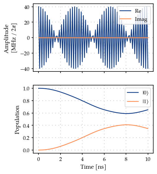
As expected, we get a partial transfer and a low fidelity.

print(f"State fidelity: {zeroone.measure(times)}")

State fidelity: 0.34736071270511687

Optimization

We define an optimizer and link our fidelity measure as a goal function and the parameters of the cosine tone.

optmap = OptimizationMap()
optmap.add(gen, [params_gen[0], params_gen[2]])
opt = ScipyOptimizer(zeroone, optimization_map=optmap)

One might think that the gradient associated with controlled_qubit would not be empty, but instead

controlled_qubit.get_gradient_at_timestep(np.array([t_simu]))

Array([], shape=(0, 2, 2), dtype=float64)

This is because, the parameters have been passed, but not “registered” by optmap. To remedy this

optmap.register_params_with_optimizables()
print(controlled_qubit.get_gradient_at_timestep(np.array([t_simu])))

[[[-0.        +0.j        -0.49605735+0.j       ]
  [-0.49605735+0.j        -0.        +0.j       ]]

 [[ 0.        -0.j        -0.15749839-1.2467281j]
  [-0.15749839-1.2467281j  0.        -0.j       ]]]

tone.get_value_and_gradient([t_simu])

(Array(2.51327412e+08, dtype=float64), Array([[1.]], dtype=float64))

In this case, as expected, we get two matrices which represent the gradient of the qubit Hamiltonian with respect to the two parameters we want to optimize, which can be accessed via the optmap as

print(optmap.get_all_parameters())

[Amplitude: 40 MHz x 2pi, lo_freq: 4.85 GHz x 2pi]

We can now run the optimization as

print(opt.optimize(times))

{'status': 1, 'value': 3.008704396734174e-13, 'iterations': 33, 'message': 'CONVERGENCE: NORM OF PROJECTED GRADIENT <= PGTOL'}

The new optimal parameters are

print(optmap.get_all_parameters())

[Amplitude: 50.2 MHz x 2pi, lo_freq: 4.8 GHz x 2pi]

We can now plot the optimized dynamics

plot_signal_and_dynamics(gen, prop, ts, state_labels=[r"$|0\rangle$", r"$|1\rangle$"]);

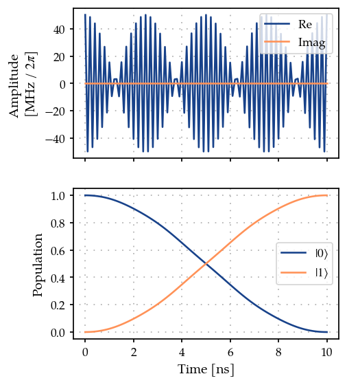
We can see from the plot and optimizer output that we have found good controls.

print(f"State fidelity: {zeroone.measure(times)}")

State fidelity: 0.9999999999996274

In this notebook, we focused on state preparation. In the next notebook, we will show how to perform the optimization directly in terms of gate fidelity.