Single spin Part 2: Gradient descent gate optimization

In this notebook, we show how to use ParaQeet to optimize a single-qubit gate, specifically an \(X\)-gate.

import matplotlib.pyplot as plt
import numpy as np

from paraqeet.measurement.unitary_fidelity import UnitaryFidelity
from paraqeet.model.closed_system import ClosedSystem
from paraqeet.model.drive_operator import DriveOperator
from paraqeet.model.qubit import Qubit
from paraqeet.optimization_map import OptimizationMap
from paraqeet.optimizers.scipy_optimizer import ScipyOptimizer
from paraqeet.optimizers.scipy_optimizer_gradient import ScipyOptimizerGradient
from paraqeet.propagation.scipy_expm_goat import ScipyExpmGOAT
from paraqeet.quantity import Quantity
from paraqeet.signal.envelopes import ConstantEnvelope
from paraqeet.signal.iq_mixer import IQMixer

System Setup

We first set up the qubit system we want to control. We set the qubit frequency \(\omega_q / 2 \pi\) to be \(4.327884\) GHz and define the Hamiltonian as

\[H(t)=H_\text{drift}+H_c(t)= \frac{\omega_q}{2} \sigma_z + \Omega(t)\sigma_x,\]

where \(\Omega(t)\) will be supplied by the generator.

freq = 4.327884e9 * 2 * np.pi

# drive = DriveOperator(gen, is_longitudinal=False)
controlled_qubit = Qubit(
    frequency=Quantity(
        freq,
        min_value=freq / 4,
        max_value=freq,
        unit="Hz",
        name="Qubit frequency",
    ),
    drives=[],
)

For signal generation, we define a simple cosine shaped tone generator \(A \cos(\omega t)\)

t_simu = 10e-9
tone = ConstantEnvelope()
# In this notebook we set the parameter t_final equal to the simulation
# time, but it is not strictly necessary as long as t_final is larger
# than t_simu (see the notebook 02A_Single_qubit_state_preparation.ipynb)
tone.t_final.set_value(t_simu)
gen = IQMixer(envelopes=[tone])

We can inspect the parameters with

params_tone = tone.get_parameters()
print(params_tone)
params_gen = gen.get_parameters()
print(params_gen)

[Amplitude: 24.7 MHz x 2pi, t_final: 10 ns]
[Amplitude: 24.7 MHz x 2pi, t_final: 10 ns, lo_freq: 4.8 GHz x 2pi, Phase: 0 rad]

In this notebook, we would like to optimize the amplitude Amplitude and frequency lo_freq if the drive. We add a drive on the qubit.

drive = DriveOperator(gen, is_longitudinal=False)
controlled_qubit.drives = [drive]
model = ClosedSystem(controlled_qubit)

In this notebook, we would like to optimize the amplitude Amplitude and frequency lo_freq if the drive. We add a drive on the qubit.

drive = DriveOperator(gen, is_longitudinal=False)
controlled_qubit.drives = [drive]
model = ClosedSystem(controlled_qubit)

Textbook values for implementing an \(X\) rotation on this system at a time \(T\) would be \(\omega=\omega_q\) and \(A=\pi/T\). We use some offset from these values as initial guess to demonstrate the optimization procedure.

params_gen[0].set_value(0.5 * np.pi / t_simu)
params_gen[2].set_value(1.01 * freq)

We select a propagation method, piecewise constant exponentiation, and configure an \(X\)-gate as a target gate. Also we initialize the identity at time \(0\).

prop = ScipyExpmGOAT(model, resolution=500e9)
times = np.array([0.0, t_simu])

pauli_x = np.array([[0.0, 1.0], [1.0, 0.0]])
pauli_y = np.array([[0.0, -1.0j], [1.0j, 0.0]])
pauli_z = np.array([[1.0, 0.0], [0.0, -1.0]])

prop.set_initial_state(np.identity(2))
gate_fid = UnitaryFidelity(
    propagation=prop,
    gate=pauli_x,
)

from plotting import plot_signal_and_dynamics

ts = np.linspace(0.0, t_simu, 501)
plot_signal_and_dynamics(gen, prop, ts, state_labels=[r"$|0\rangle$", r"$|1\rangle$"]);

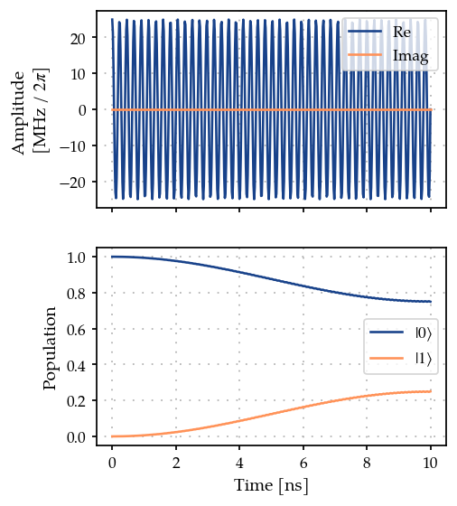
As expected, we get a partial transfer and a low fidelity.

print(f"Gate fidelity: {gate_fid.measure(times)}")

Gate fidelity: 0.09555411208408474

We define an optimizer and link our fidelity measure as a goal function and the parameters of the cosine tone and optimize just amplitude and frequency, as in the state transfer example.

optmap = OptimizationMap()
optmap.add(gen, [params_gen[0], params_gen[2]])
opt = ScipyOptimizerGradient(gate_fid, optimization_map=optmap)

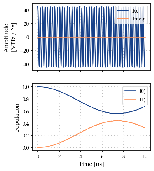
opt.optimize(times)

{'status': 1, 'value': 0.8037201693294315, 'iterations': 17, 'message': 'CONVERGENCE: NORM OF PROJECTED GRADIENT <= PGTOL'}

plot_signal_and_dynamics(gen, prop, ts, state_labels=[r"$|0\rangle$", r"$|1\rangle$"]);

Dynamics of Pauli operators

Here, we end up with an unsatisfactory result. For optimizing gate fidelities, looking at state populations does not give enough information to identify the problem.

def expecation_value(op, states):
    """Get the expectation value across states."""
    ex = []
    for state in states:
        ex.append(np.real(state.conj() @ op @ state.T))
    return ex

def plot_pauli():
    """Plot the Pauli operators."""
    ts = np.linspace(0, t_simu, 1001)
    states = prop.propagate(ts)
    sig = gen.get_value(ts) / 1e6 / (2 * np.pi)

    fig, ax = plt.subplots(2, figsize=(4, 4), sharex=True)
    ax[0].plot(ts / 1e-9, sig)
    ax[0].set_ylabel(r"Field [MHz / $2\pi$]")
    ax[0].grid(True, linestyle=(1, (1, 5)), linewidth=1)

    ax[1].plot(ts / 1e-9, expecation_value(pauli_x, states[:, :, 0]))
    ax[1].plot(ts / 1e-9, expecation_value(pauli_y, states[:, :, 0]))
    ax[1].plot(ts / 1e-9, expecation_value(pauli_z, states[:, :, 0]))
    ax[1].set_ylabel(r"Expectation value $\langle\hat\sigma_i\rangle$")
    ax[1].grid(True, linestyle=(1, (1, 5)), linewidth=1)

    ax[-1].set_xlabel("Time [ns]")
    ax[1].legend(["X", "Y", "Z"])
    return fig, ax


plot_pauli()

(<Figure size 500x500 with 2 Axes>,
 array([<Axes: ylabel='Field [MHz / $2\pi$]'>,
        <Axes: xlabel='Time [ns]', ylabel='Expectation value $\langle\hat\sigma_i\rangle$'>],
       dtype=object))

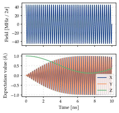
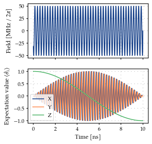
Instead, we look at the expectation values of the three Pauli operators and observe that the qubit is rotating at its eigenfrequency along the Z-axis. We can mitigate this problem by allowing the rotation axis of our drive to shift and include the phase parameter in the optimization.

optmap = OptimizationMap()
optmap.add(tone, [params_gen[0], params_gen[2], params_gen[3]])
opt = ScipyOptimizer(gate_fid, optimization_map=optmap)

params_gen[0].set_value(0.5 * np.pi / t_simu)
params_gen[2].set_value(1.01 * freq)
opt.optimize(times)

{'status': 1, 'value': 1.0475176281943277e-11, 'iterations': 108, 'message': 'CONVERGENCE: RELATIVE REDUCTION OF F <= FACTR*EPSMCH'}

plot_pauli()

(<Figure size 500x500 with 2 Axes>,
 array([<Axes: ylabel='Field [MHz / $2\pi$]'>,
        <Axes: xlabel='Time [ns]', ylabel='Expectation value $\langle\hat\sigma_i\rangle$'>],
       dtype=object))